6. Bessel Processes Part I

The purpose of these notebooks (Bessel Processes Part I-III) is to provide an illustration of the Bessel Processes and some of their main properties.

• In Part I, we introduce both Bessel and Squared Bessel processes with integer dimension \(d\geq 2,\) and study some of its main properties.

• In Part II, we show that Bessel processes with integer dimension satisfy certain Stochastic Differential Equations (SDEs). This representation allows us to extend them to the non-integer case.

• Finally, in Part III we illustrate both Bessel and Squared Bessel processes with general dimension \(\delta \geq 0\), and some of its main properties.

Before diving into the theory, let’s start by loading the libraries

• aleatory

• matplotlib

together with the style sheet Quant-Pastel Light.

from aleatory.processes import BESProcess, BESQProcess
import matplotlib.pyplot as plt
quant_pastel = "https://raw.githubusercontent.com/quantgirluk/matplotlib-stylesheets/main/quant-pastel-light.mplstyle"
plt.style.use(quant_pastel)
plt.rcParams["figure.figsize"] = (12,6)

These tools will help us to make insightful visualisations of Bessel processes.

Important

In Part I, we will focus on the Bessel processes with integer dimension \(d\geq 2\), and starting at zero. In the following parts, we will cover how to generalise these two conditions.

6.1. Definition

Let \(W =\{ W_t = (W^1_t, \cdots, W^d_t) : t\geq 0 \},\) be a \(d\)-dimensional standard Brownian Motion, for some integer \(d \geq 2\).

The Bessel process of dimension \(d\), is defined as the Euclidean norm of \(W\). That is

(6.1)\[\begin{equation} X_t = \|W_t\| = \sqrt{\sum_{i=1}^d (W^i_t)^2}, \qquad t \geq 0. \end{equation}\]

Similarly, the Squared Bessel process of dimension \(d\), is defined as the squared Euclidean norm of \(W\).

(6.2)\[\begin{equation} Y_t = \|W_t\|^2 = \sum_{i=1}^d (W^i_t)^2, \qquad t \geq 0. \end{equation}\]

Notation

Hereafter, we will use the following notation:

• \(BES_0^d\) : to denote a Bessel process of dimension \(d\) starting at zero, as defined in equation (6.1)

• \(BES_0^d\) : to denote a Squared Bessel process of dimension \(d\) starting at zero, as defined in equation (6.2)

6.2. Simulation

The previous definitons (in terms of a multidimensional Brownian Motion) allow us to simulate paths from Bessel processes of integer dimension easily as follows.

6.2.1. Bessel Process

In order to simulate a path from a Bessel process with integer dimension \(d\geq 2\), let us start by taking a discrete partition over an interval \([0,T]\) for the simulation to take place. For simplicity, we are going to take an equidistant partition of size \(n\in \mathbb{N}\), over the interval \([0,T]\), i.e.:

\[\begin{equation*} t_j = \frac{j}{n-1} T, \qquad \hbox{for } j = 0, \cdots, n-1. \end{equation*}\]

Then, the goal is to simulate a path of the form

\[X_{t_j} = \| W_{t_j} \|, \quad j=0,\cdots, n-1,\]

where \(W\) denotes a \(d\)-dimensional Brownian motion. To do this, we follow the next steps:

• Step 1. For \(i=1, \cdots, d\):

  Simulate a path of the form

  \[\{ W_{t_j}^{i} , j=0,\cdots, n-1\},\]

  That is, we simulate from \(d\) independent standard Brownian motions. See Brownian Motion for details on how to simulate from a standard Brownian motion. This allows us to construct the vectors

\[\begin{equation*} W_{t_j} = (W_{t_j}^1, \cdots W_{t_j}^d), \qquad j=1,\cdots\ n. \end{equation*}\]

• Step 2. For \(j=1,\cdots\ n\):

  Take the norm of such vectors, that is

  \[\begin{equation*} X_{t_j} = \sqrt{ \sum_{i=1}^d (W_{t_j}^{i})^2 }. \end{equation*}\]

# Snippet to simulate a path from a Bessel process with integer dimension
from aleatory.processes import BrownianMotion
import numpy as np

d = 3
T = 1.0
n = 100

times = np.linspace(0, T, n) # Partition of the interval [0,T]
brownian = BrownianMotion(T) # A Brownian Motion instance

brownian_samples = [brownian.sample_at(times) for _ in range(d)] # Step 1. Building the vectors (W_{t_j}^1 , ... W_{t_j}^d)
bessel_path = np.array([np.linalg.norm(coord) for coord in zip(*brownian_samples)]) # Step 2. Taking the Euclidian norm

Now, let’s plot our simulated path!

plt.plot(times, bessel_path, 'o-', lw=1)
plt.title('Bessel Process Path')
plt.show()

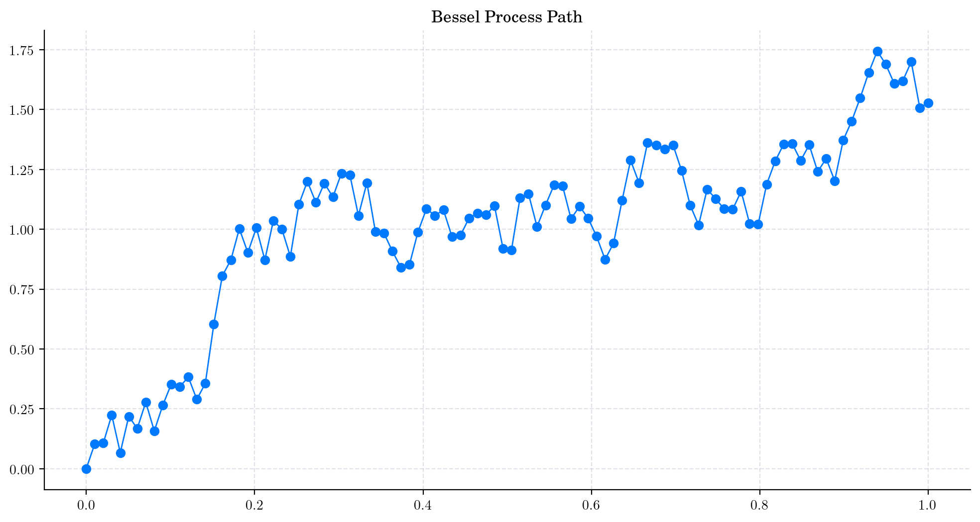
Note

In this plot, we are using a linear interpolation to draw the lines between the simulated points.

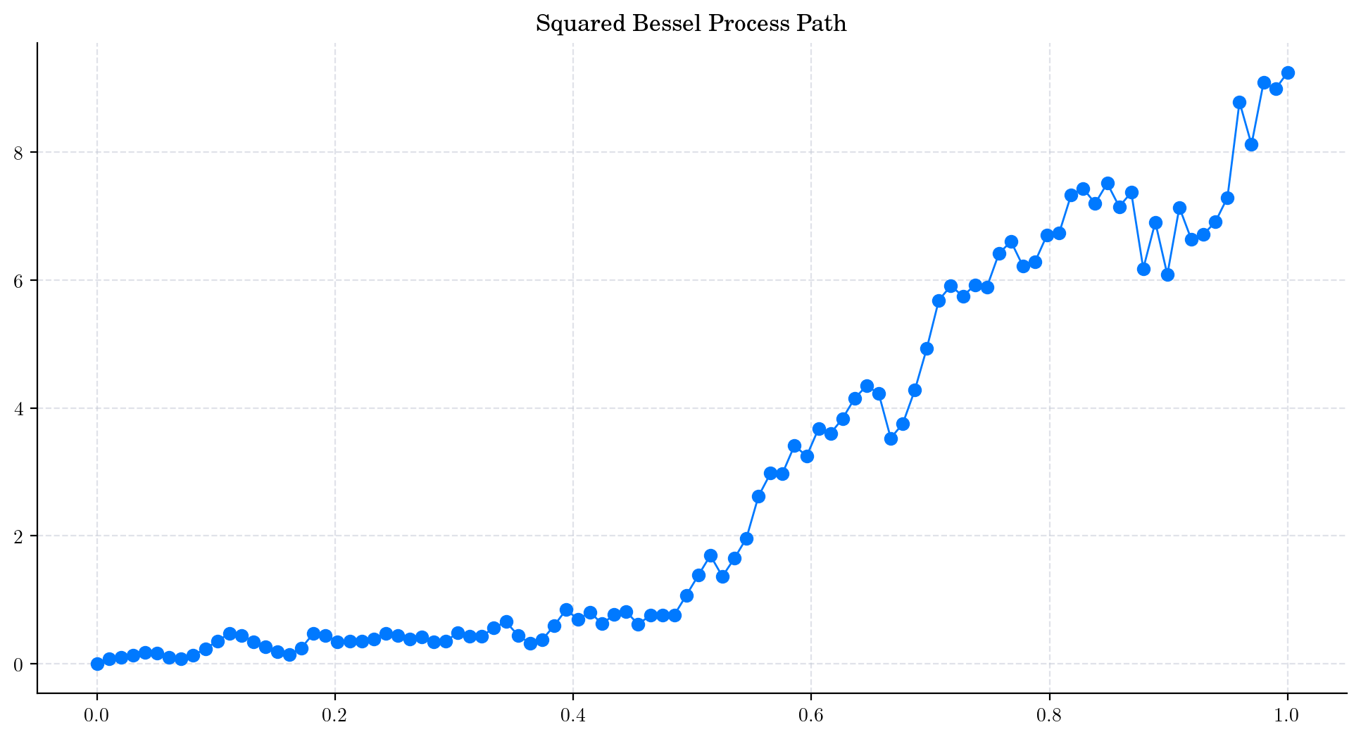
6.2.2. Squared Bessel Process

We can follow the same logic to simulate a path from a Squared Bessel process. The only differences is the calculation in Step 2. Instead of calculating the norm we just get the squared norm, i.e.:

\[\begin{equation*} Y_{t_j} = \sum_{i=1}^d (W_{t_j}^{i})^2 , \qquad j=1,\cdots\ n. \end{equation*}\]

Let’s write this in Python.

# Snippet to simulate a path from a Squared Bessel process with integer dimension
d = 4
T = 1.0
n = 100

times = np.linspace(0, T, n) # Partition of the interval [0,T]
brownian = BrownianMotion(T) # A Brownian Motion instance

brownian_samples = [brownian.sample_at(times) for _ in range(d)] # Step 1. Building the vectors (W_{t_j}^1 , ... W_{t_j}^d)
bessel_path = np.array([(np.linalg.norm(coord))**2 for coord in zip(*brownian_samples)]) # Step 2 (Modified). Taking the Square of the Euclidian norm

plt.plot(times, bessel_path, 'o-', lw=1) # Plot the path
plt.title('Squared Bessel Process Path')
plt.show()

6.2.3. Simulating and Visualising Paths

To simulate several paths from Bessel and Squared Bessel processes and visualise them we can use the methods simulate and plot from the aleatory library.

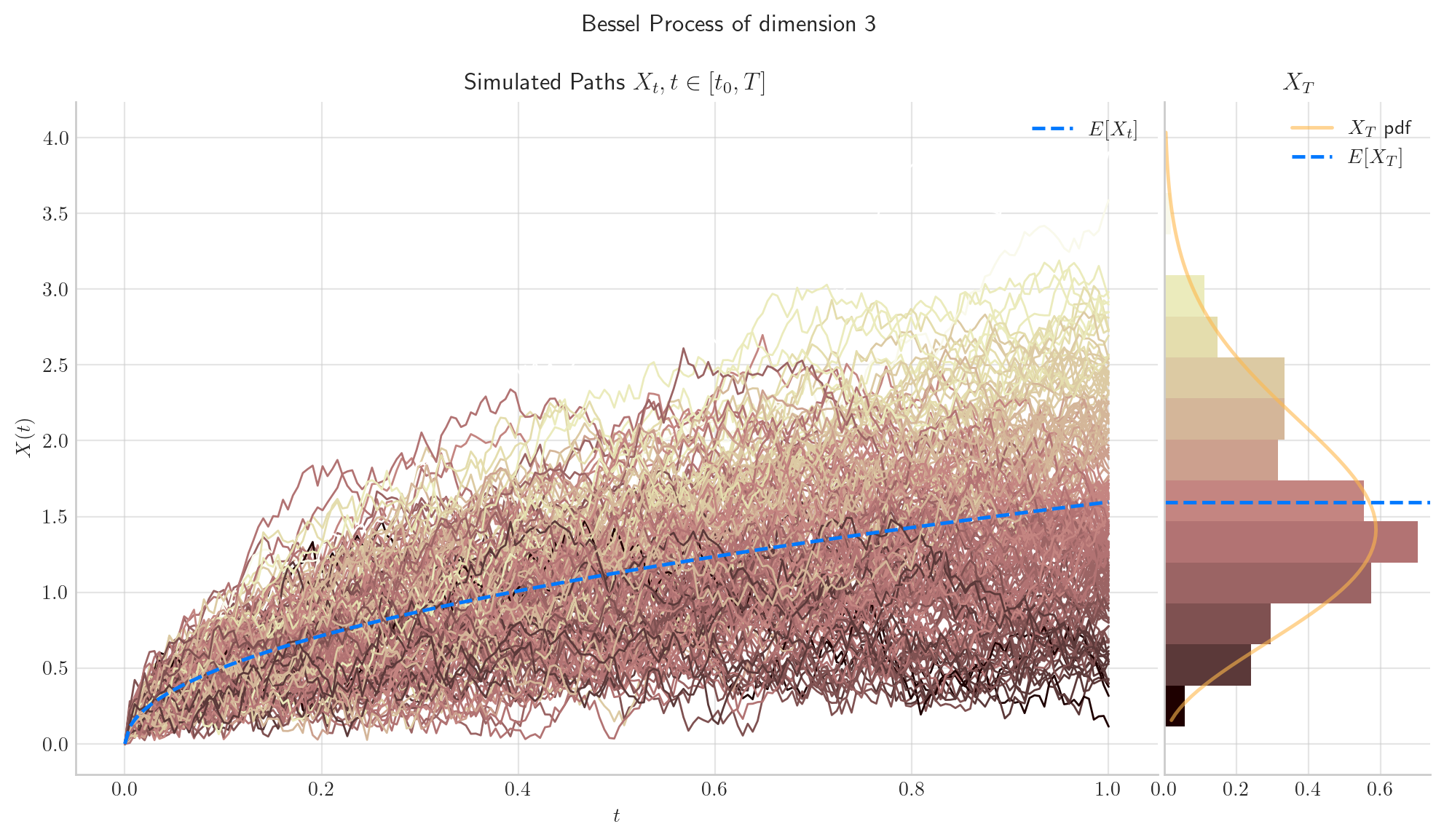
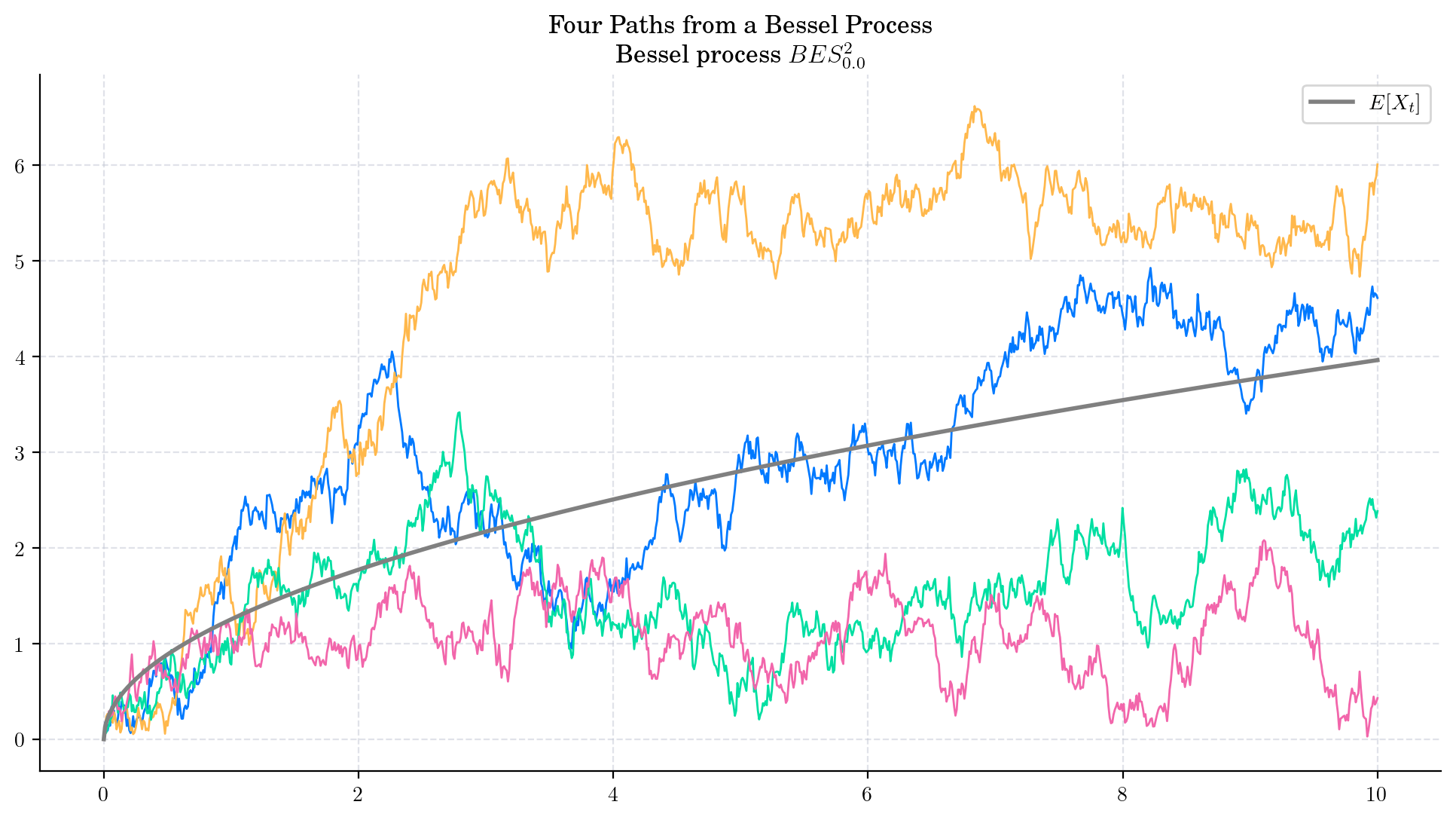
Let’s simulate 5 paths from a Bessel Process of dimension 3, over the interval \([0,1]\) using a partition of 100 points.

Tip

Remember that the number of points in the partition is defined by the parameter \(n\), while the number of paths is determined by \(N\).

The following snippet simulates the paths and returns them as a numpy array object.

# Snippet to Simulate N paths from the Bessel process
from aleatory.processes import BESProcess
bes = BESProcess(dim= 3)
paths = bes.simulate(n=100, N=5)

If we want to simulate and visualise the paths, we will use the method plot from the aleatory library.

# Snippet to Simulate and Visualise the paths from the Bessel process
from aleatory.processes import BESProcess
bes = BESProcess(dim= 3)
fig = bes.plot(n=100, N=5)

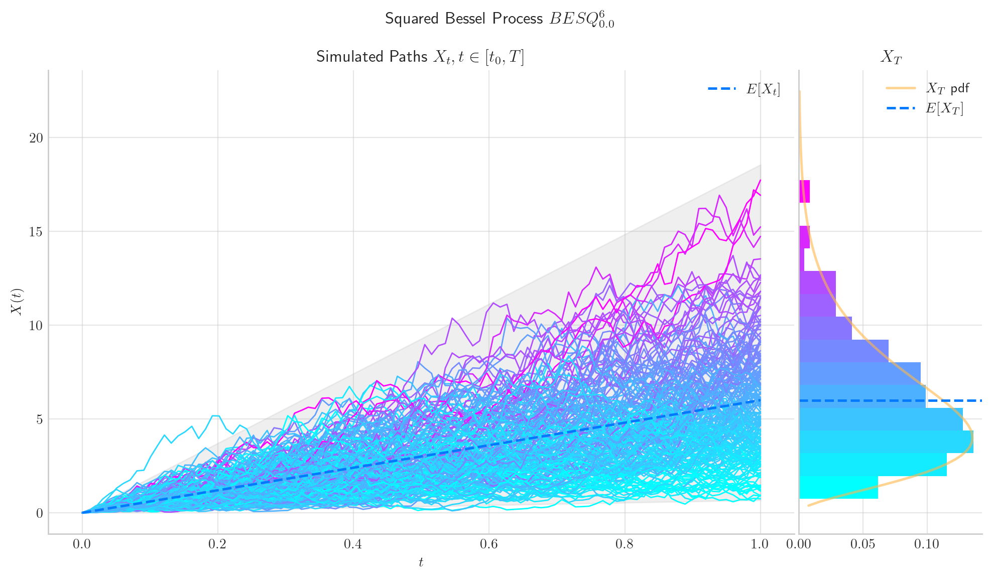
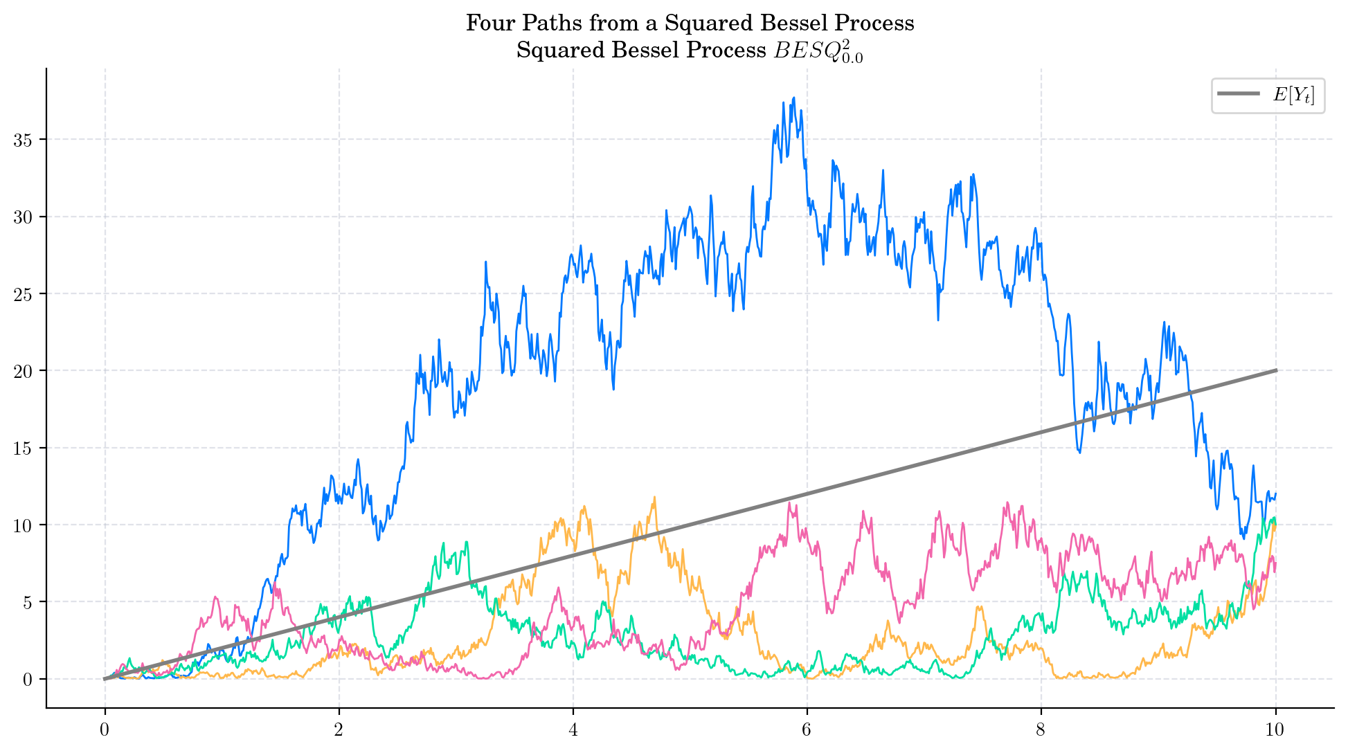
Similarly, let’s simulate 5 paths from a Squared Bessel process of dimension 6, over the interval \([0,1]\) using a partition of 100 points.

# Snippet to Simulate and Visualise the paths from the Squared Bessel process
from aleatory.processes import BESQProcess
bes = BESQProcess(dim= 6)
fig = bes.plot(n=100, N=5)

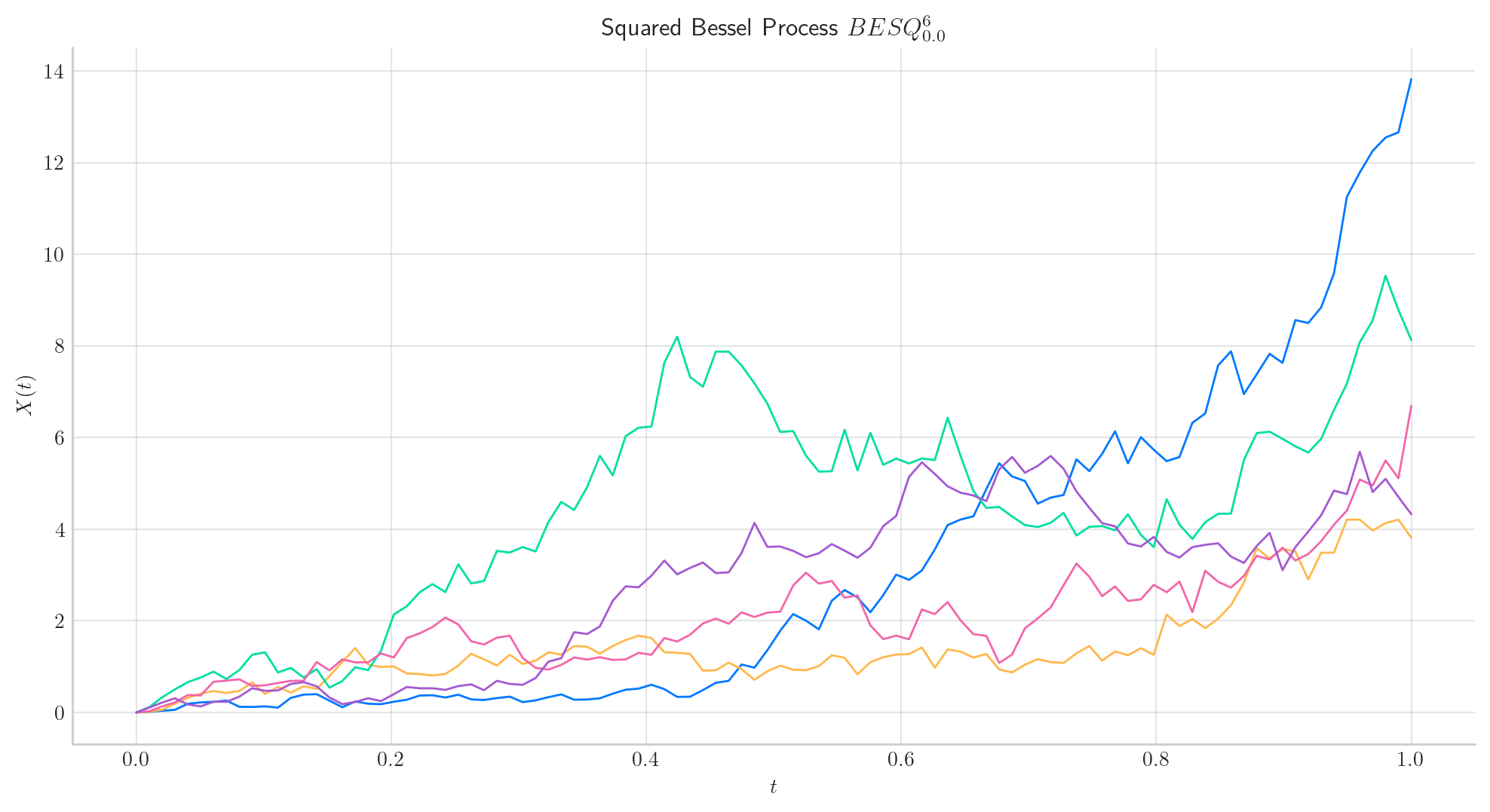
Note

In all plots we are using a linear interpolation to draw the lines between the simulated points.

6.3. Marginal Distributions

For any given \(t\geq 0\), the definition of a \(d\)-dimensional Brownian Motion implies that each component \(W^i_t\), follows a normal distribution \(\mathcal{N}(0,t)\). Moreover, these components are independent of each other.

Hence, we have

(6.3)\[\begin{equation} X_t = \sqrt{t} \sqrt{ \sum_{i=1}^d \left( \dfrac{W_t^i}{ \sqrt{t}} \right)^2 } \sim \sqrt{t} \chi(d), \qquad t\geq 0, \end{equation}\]

i.e.; the marginal distribution of a Bessel process \(BES_0^d\) (with integer dimension \(d\geq2\)) is a scaled Chi random-variable with \(d\)-degrees of freedom.

Similarly,

(6.4)\[\begin{equation} Y_t = \sum_{i=1}^d (W^i_t)^2 = t \sum_{i=1}^d \left( \dfrac{W_t^i}{\sqrt{t}} \right)^2 \sim t \chi^2(d), \qquad t\geq 0, \end{equation}\]

that is, the marginal distribution of a Squared Bessel process \(BESQ_0^2\) (with integer dimension \(d\geq 2\)) is a scaled Chi-squared with \(d\)-degrees of freedom.

Note

• The number of degrees of freedom \(d\) does not depend on \(t\), which means that the number of degrees of freedom remains constant as the process evolves.

6.3.1. Expectation and Variance

6.3.1.1. Bessel

For each \(t>0\), the marginal distribution \(X_t|X_0=0\) from a Bessel process \(BES_0^d\), with integer dimension \(d\geq 2\), satisfies

\[\begin{equation*} \mathbf{E}[X_t] = \mathbf{E}\left[ \sqrt{t} \sqrt{ \sum_{i=1}^d \left( \dfrac{W_t^i}{ \sqrt{t}} \right)^2 } \right]= \sqrt{2t} \dfrac{\Gamma (\frac{d+1}{2})}{\Gamma (\frac{d}{2})} , \end{equation*}\]

and

\[\begin{equation*} \mathbf{Var} [X_t ] = \mathbf{Var}\left[\sqrt{t} \sqrt{ \sum_{i=1}^d \left( \dfrac{W_t^i}{ \sqrt{t}} \right)^2 } \right]= t d - \mathbf{E}[X_t]^2 = td - 2t \left( \dfrac{\Gamma (\frac{d+1}{2})}{\Gamma (\frac{d}{2})} \right)^2, \end{equation*}\]

6.3.1.1.1. Python Implementation

For given \(d\geq 2, t\geq 0\), we can implement the above formulas for the expectation, and variance, as follows.

from scipy.special import gamma
from math import sqrt
d = 3
t= 2

expectation = sqrt(2*t)*gamma((d+1)/2)/gamma(d/2) 
variance = t*d - expectation**2

print(f'For d={d}' , f't={t}', sep=", ")
print(f'E[X_t] = {expectation: .6f}')
print(f'Var[X_t] = {variance :.14f}')

For d=3, t=2
E[X_t] =  2.256758
Var[X_t] = 0.90704182105935

Alternatively, we can use the method get_marginal to obtain the marginal distribution and the get its mean and variance

from aleatory.processes import BESProcess
d = 3
t= 2
bes = BESProcess(dim=d)
marginal = bes.get_marginal(t=t)
print(marginal.mean())
print(marginal.var())

2.2567583341910256
0.9070418210593473

6.3.1.2. Squared Bessel

For each \(t>0\), the conditional marginal \(Y_t|Y_0=0\) from a Squared Bessel process starting from zero with integer dimension \(d\geq 2\), satisfies

\[\begin{equation*} \mathbf{E}[Y_t] = \mathbf{E}\left[ t \sum_{i=1}^d \left( \dfrac{W_t^i}{\sqrt{t}} \right)^2\right]= t d , \end{equation*}\]

and

\[\begin{equation*} \mathbf{Var} [Y_t ] = \mathbf{Var}\left[ t \sum_{i=1}^d \left( \dfrac{W_t^i}{\sqrt{t}} \right)^2\right]= t^2 2d , \end{equation*}\]

6.3.1.2.1. Python Implementation

For given \(d\geq 2, t\geq 0\), we can implement the above formulas for the expectation, and variance, as follows.

d = 3
t= 2

expectation = t*d
variance = (t**2)*(2*d) 
print(f'For d={d}' , f't={t}', sep=", ")
print(f'E[Y_t] = {expectation: .6f}')
print(f'Var[Y_t] = {variance :.6f}')

# from aleatory.processes import BESProcess
bes = BESQProcess(dim=d)
marginal = bes.get_marginal(t=t)
print(marginal.mean())
print(marginal.var())

For d=3, t=2
E[Y_t] =  6.000000
Var[Y_t] = 24.000000
6.0
24.0

6.3.2. Probability Density Functions

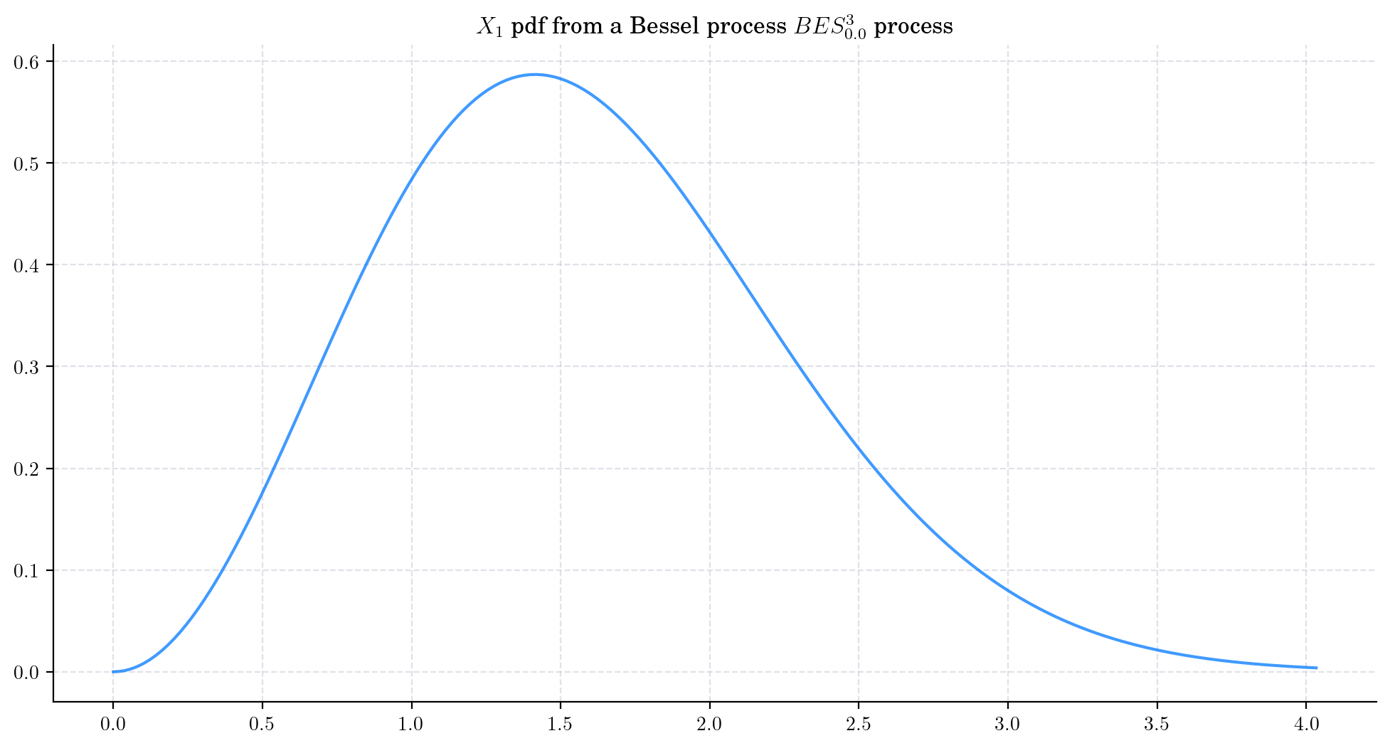
The probability density function (pdf)of the marginal distribution \(X_t\), from a Bessel process with integer dimension \(d\geq 0\), is given by the following expression

(6.5)\[\begin{equation} f_X(x, t) = \frac{1}{2^{\frac{d}{2}-1} \Gamma\left(\frac{d}{2}\right) \sqrt{t}} \left(\frac{x}{\sqrt{t}}\right)^{d -1} e^{-\frac{x^2}{2 t}}, \qquad x, t>0. \end{equation}\]

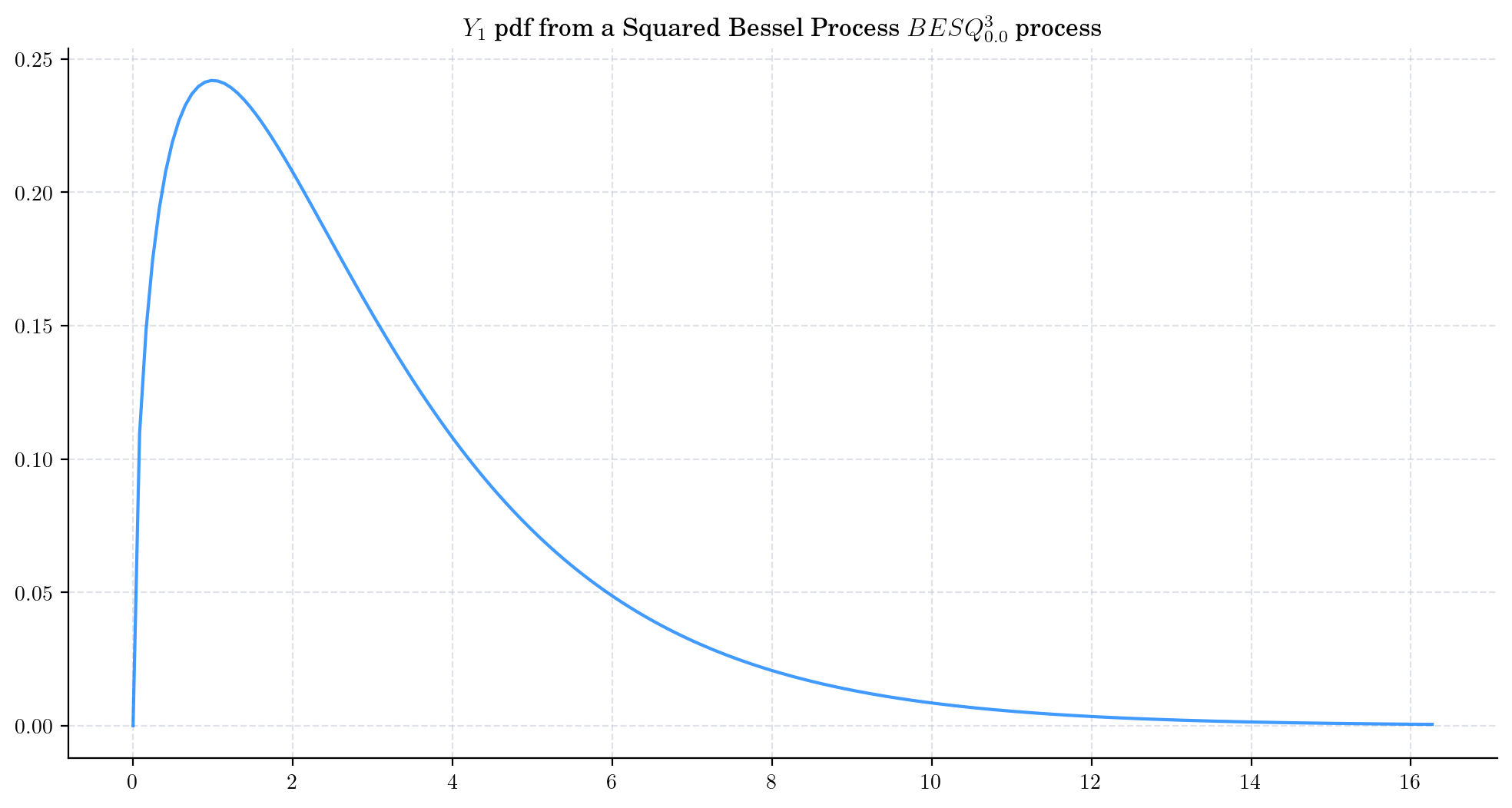
The probability density function (pdf)of the marginal distribution \(Y_t\), from a Squared Bessel process with integer dimension \(d\geq 0\), is given by the following expression

(6.6)\[\begin{equation} f_Y(y, t) = \frac{1}{2^{\frac{d}{2}} \Gamma\left(\frac{d}{2}\right) t} \left(\frac{y}{t}\right) ^{\frac{d}{2} -1} e^{-\frac{y}{2 t}}, \qquad y, t>0. \end{equation}\]

6.3.2.1. Visualisation

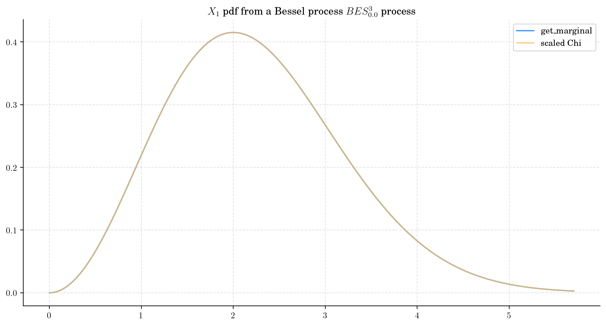
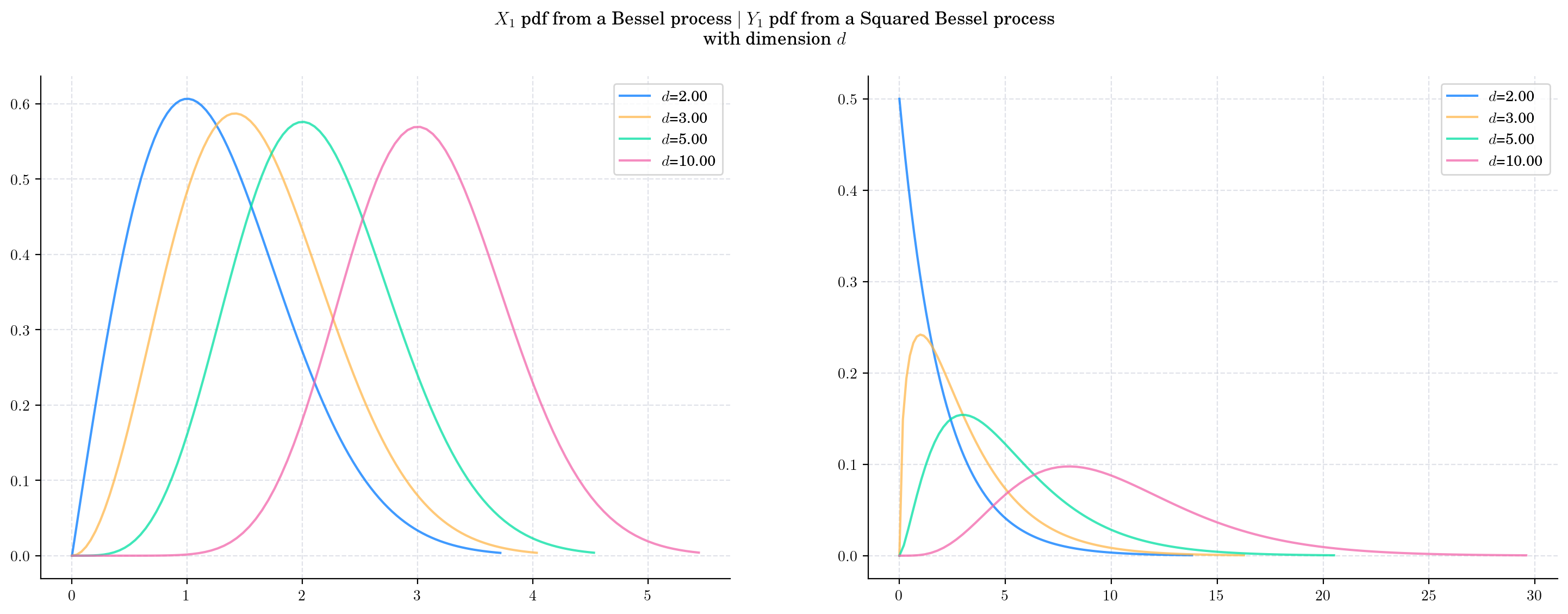
To visualise these probability density functions in Python, we can use the method get_marginal from the aleatory library. Let’s consider a Bessel process BESProcess(dim=3) and plot the density function of the marginal \(X_1\)

# from aleatory.processes import BESProcess
process = BESProcess(dim= 3)
X_1 = process.get_marginal(t=1)
x = np.linspace(0, X_1.ppf(0.999), 200)
plt.plot(x, X_1.pdf(x), '-', lw=1.5, alpha=0.75, label=f'$t$={1:.2f}')
plt.title(f'$X_1$ pdf from a ' + process.name + ' process')
plt.show()

We can also use do this by using the fact that \(X_1\) follows a Chi distribution with parameter 3. You can try this alternative method by running the following code.

# from aleatory.processes import BESProcess
# import numpy as np 
from scipy.stats import chi

d = 3
t = 2 
process = BESProcess(dim=d)
X_1 = process.get_marginal(t=t)
chi_rv = chi(3, scale=np.sqrt(t))

x = np.linspace(0, X_1.ppf(0.999), 200)
plt.plot(x, X_1.pdf(x), '-', lw=1.5, alpha=0.75, label='get_marginal')
plt.plot(x, chi_rv.pdf(x), label='scaled Chi')
plt.title(f'$X_1$ pdf from a ' + process.name + ' process')
plt.legend()
plt.show()

Similarly, we can take a Squared Bessel process BESQProcess(dim=3) and plot the density function of \(Y_1\).

# from aleatory.processes import BESQProcess
process = BESQProcess(dim= 3)
Y_1 = process.get_marginal(t=1)
y = np.linspace(0, Y_1.ppf(0.999), 200)
plt.plot(y, Y_1.pdf(y), '-', lw=1.5, alpha=0.75, label=f'$t$={1:.2f}')
plt.title(f'$Y_1$ pdf from a ' + process.name + ' process')
plt.show()

Next, we vary the value of the dimension \(d\) and plot the corresponding pdfs. As \(d\) increases:

• The density from the Bessel marginal moves towards the right and becomes more symmetric.

• The density from the Squared Bessel marginal becomes wider and the shape changes as well.

fig, axs = plt.subplots(1, 2, figsize=(18, 6))
dims = [2, 3, 5, 10]
for d in dims:
    processes = [BESProcess(dim=d), BESQProcess(dim=d)]
    for (process, ax) in zip(processes, axs):
        X_t = process.get_marginal(t=1.0)
        x = np.linspace(0, X_t.ppf(0.999), 100)
        ax.plot(x, X_t.pdf(x), '-', lw=1.5, alpha=0.75, label=f'$d$={d:.2f}')
        ax.legend()
fig.suptitle(f'$X_1$ pdf from a Bessel process $\mid$  $Y_1$ pdf from a Squared Bessel process\n with dimension $d$')
plt.show()

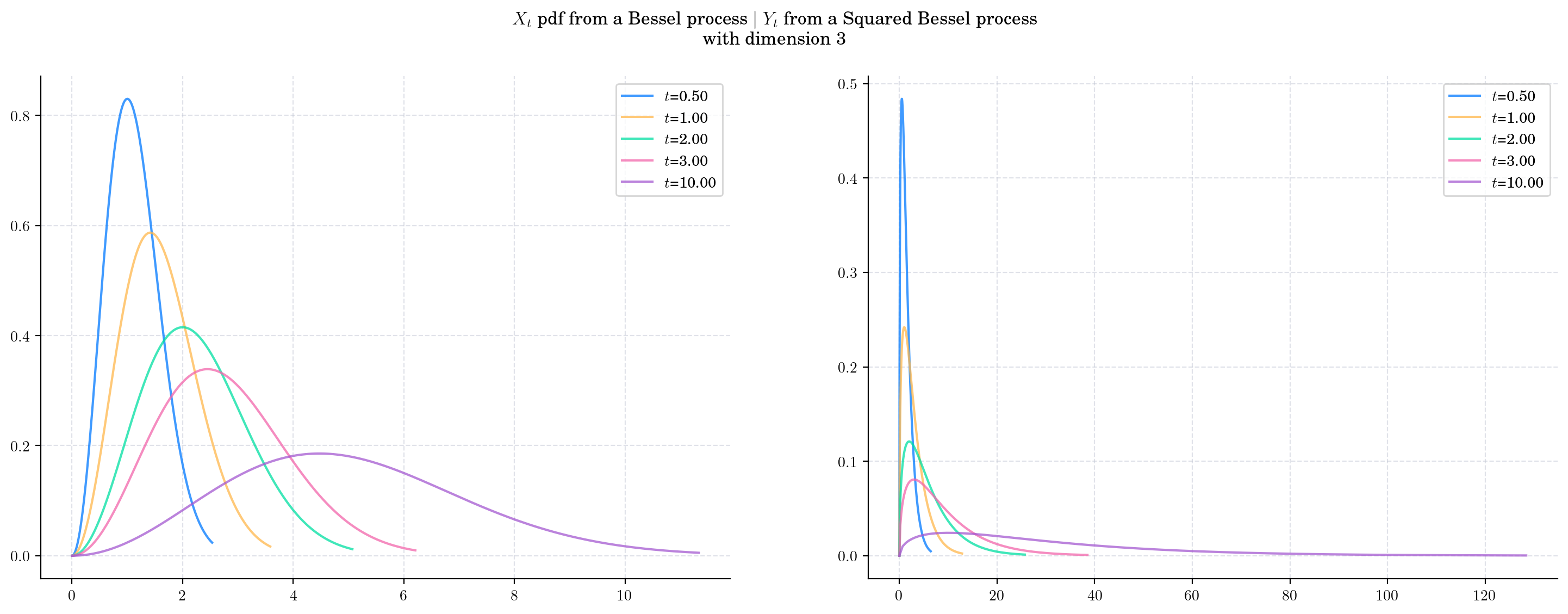
Finally, we fix the dimension (to 3) and vary the value of time \(t\) and plot the corresponding pdfs. As \(t\) increases:

• The density from the Bessel marginal moves towards the right and becomes wider. This reflects the fact that both the mean and the variance are increasing.

• The density from the Squared Bessel marginal becomes wider very rapidly as \(t\) grows.

d = 3
fig, axs = plt.subplots(1, 2, figsize=(18, 6))
t_values = [0.5,1, 2, 3, 10]

processes = [BESProcess(dim=d), BESQProcess(dim=d)]

for (process, ax) in zip(processes, axs):
        for t in t_values: 
                X_t = process.get_marginal(t=t)
                x = np.linspace(0, X_t.ppf(0.995), 200)
                ax.plot(x, X_t.pdf(x), '-', lw=1.5, alpha=0.75, label=f'$t$={t:.2f}')
                ax.legend()
fig.suptitle(f'$X_t$ pdf from a Bessel process $\mid$ $Y_t$ from a Squared Bessel process\n with dimension 3')
plt.show()

6.4. Long Time Behaviour

6.4.1. Expectation and Variance

6.4.1.1. Bessel

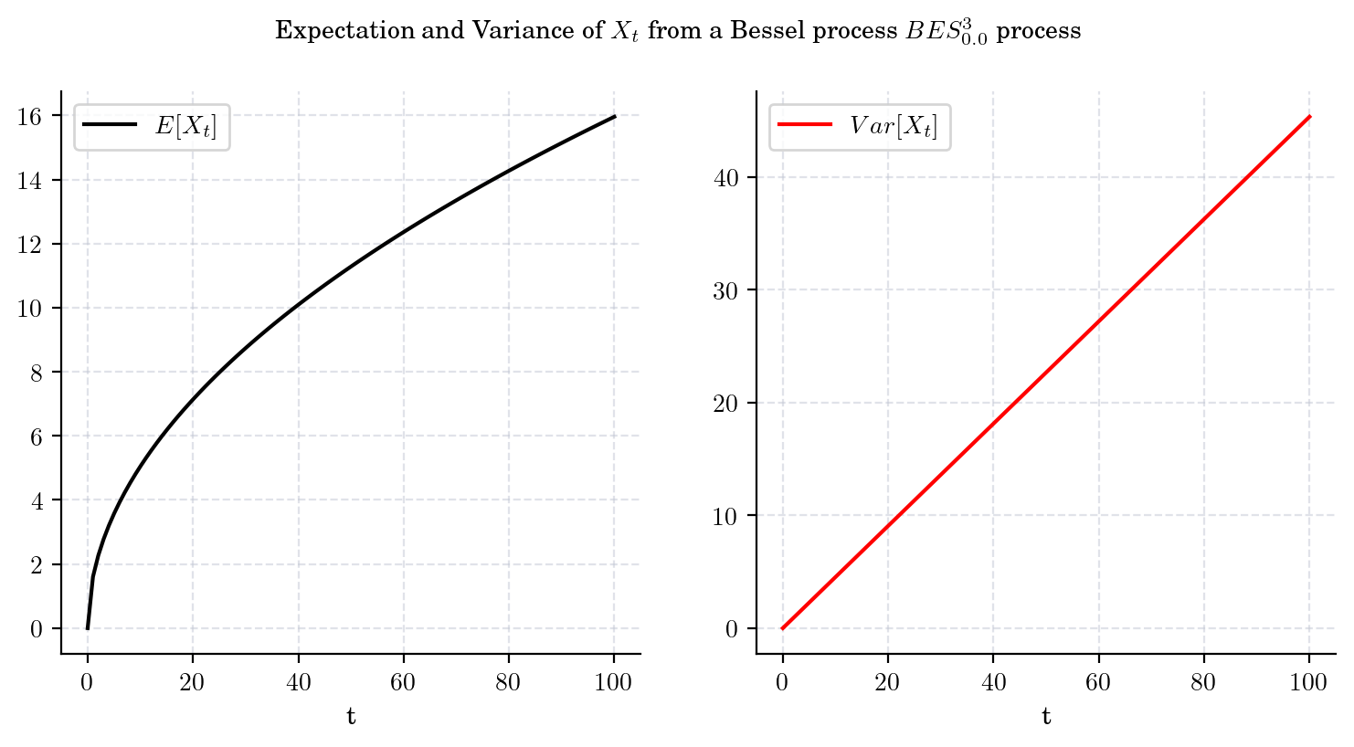
The conditional marginal from a Bessel process \(BES_0^d\), with integer dimension \(d\geq 2\), satisfies

\[\begin{equation*} \lim_{t\rightarrow \infty }\mathbf{E}[X_t] = \lim_{t\rightarrow \infty } \sqrt{2t} \dfrac{\Gamma (\frac{d+1}{2})}{\Gamma (\frac{d}{2})} = \infty, \end{equation*}\]

and

\[\begin{equation*} \lim_{t\rightarrow \infty } \mathbf{Var} [X_t ] = \lim_{t\rightarrow \infty } t \left( d- 2 \dfrac{\Gamma (\frac{d+1}{2})}{\Gamma (\frac{d}{2})} \right)^2 = \infty. \end{equation*}\]

That is, both the mean and the variance tend to infinity as \(t\) grows. Besides, these expressions imply that the variance grows faster (at linear rate with respect to \(t\)) than the mean. The next plot illustrates these observations.

def draw_mean_variance(dim=3, T=100):

    process = BESProcess(dim=dim)
    ts = np.linspace(0, T, T)
    means = process.marginal_expectation(ts)
    variances = process.marginal_variance(ts)
    fig, (ax1, ax2,) = plt.subplots(1, 2, figsize=(9, 4))
    
    ax1.plot(ts, means, lw=1.5, color='black', label='$E[X_t]$')
    ax1.set_xlabel('t')
    ax1.legend()
    ax2.plot(ts,  variances, lw=1.5, color='red', label='$Var[X_t]$')
    ax2.set_xlabel('t')
    ax2.legend()
    fig.suptitle(
        'Expectation and Variance of $X_t$ from a ' + process.name + ' process', size=10)
    plt.show()

draw_mean_variance(dim=3, T=100)

6.4.1.2. Squared Bessel

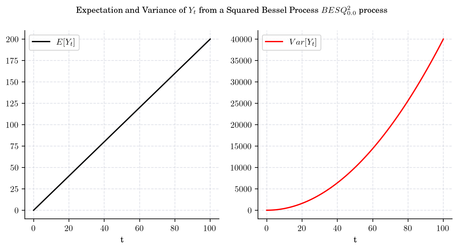
The conditional marginal from a Squared Bessel process \(BESQ_0^d\), with integer dimension \(d\geq 2\), satisfies

\[\begin{equation*} \lim_{t\rightarrow \infty }\mathbf{E}[Y_t] = \lim_{t\rightarrow \infty } td = \infty, \end{equation*}\]

and

\[\begin{equation*} \lim_{t\rightarrow \infty } \mathbf{Var} [Y_t ] = \lim_{t\rightarrow \infty } t^2 2d = \infty. \end{equation*}\]

That is, both the mean and the variance tend to infinity as \(t\) grows. Besides, from these equations we can conclude that the variance grows faster than the mean. The next plot illustrates these observations.

def draw_mean_variance(dim=3, T=100):

    process = BESQProcess(dim=dim)
    ts = np.linspace(0.00001, T, T)
    means = process.marginal_expectation(ts)
    variances = process.marginal_variance(ts)
    fig, (ax1, ax2,) = plt.subplots(1, 2, figsize=(9, 4))
    
    ax1.plot(ts, means, lw=1.5, color='black', label='$E[Y_t]$')
    ax1.set_xlabel('t')
    ax1.legend()
    ax2.plot(ts,  variances, lw=1.5, color='red', label='$Var[Y_t]$')
    ax2.set_xlabel('t')
    ax2.legend()
    fig.suptitle(
        'Expectation and Variance of $Y_t$ from a ' + process.name + ' process', size=10)
    plt.show()

draw_mean_variance(dim=2, T=100)

6.4.2. Marginal

From equations (6.3) and (6.4) we have:

\[X_t \sim \sqrt{t} \chi (d) \rightarrow \infty, \qquad \hbox{as } t\rightarrow \infty,\]

and

\[Y_t \sim t \chi^2(d) \rightarrow \infty, \qquad \hbox{as } t\rightarrow \infty.\]

The following charts illustrate this behaviour.

In particular, we can see that both the probability density functions corresponding to \(X_t\), and \(Y_t\), become flatter and wider as \(t\) grows.

d = 3
fig, axs = plt.subplots(1, 2, figsize=(18, 6))
t_values = [100, 500, 1000, 5000]
processes = [BESProcess(dim=d), BESQProcess(dim=d)]

for (process, ax) in zip(processes, axs):
    for t in t_values:
        X_t = process.get_marginal(t=t)
        x = np.linspace(0, X_t.ppf(0.995), 200)
        ax.plot(x, X_t.pdf(x), '-', lw=1.5,
                alpha=0.75, label=f'$t$={t:.0f}')
        ax.legend()
fig.suptitle(
    f'$X_t$ pdf from a $BES_0^3$ process $\mid$ $Y_t$ pdf from a $BESQ_0^3$ process')
plt.show()

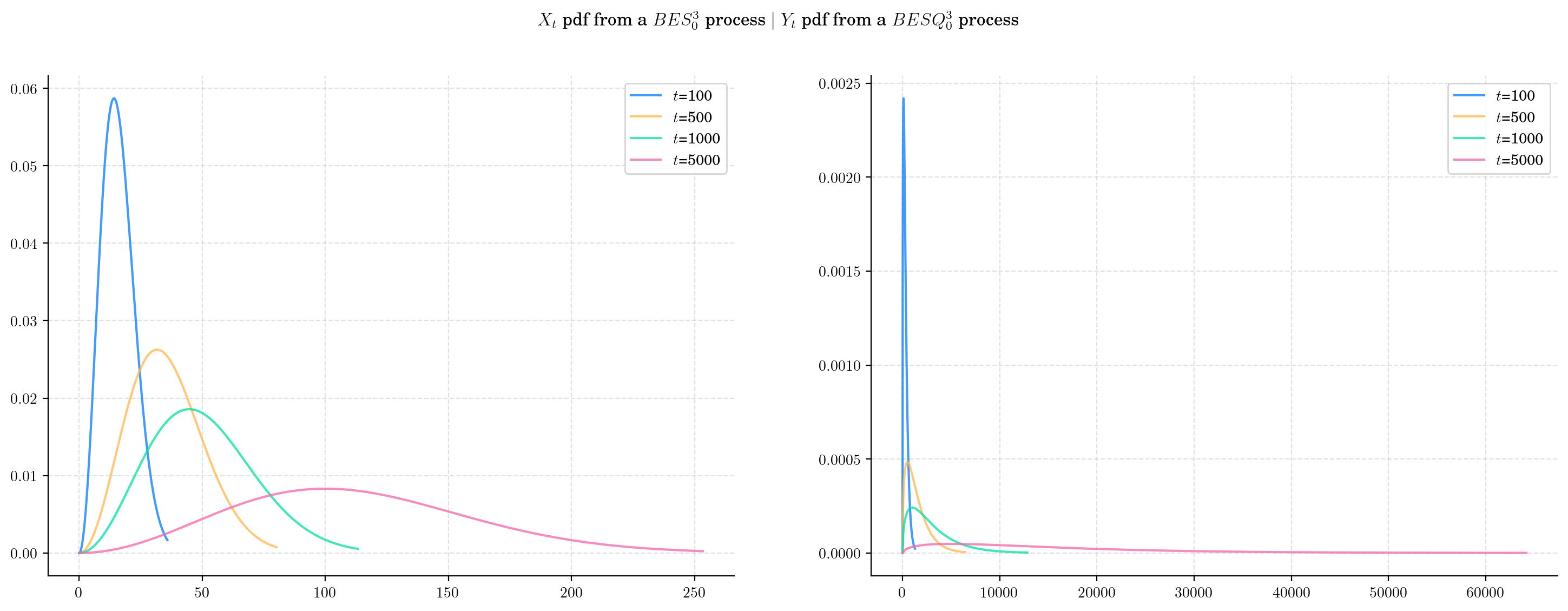
The following two charts show simulations from processes \(BES_0^3,\) and \(BESQ_0^3\), over the interval \([0,5000]\). In both cases, the plots illustrate the described long time behaviour.

# from aleatory.processes import BESProcess
bes = BESProcess(dim=3, T=5000)
fig = bes.draw(n=100, N=100)

# from aleatory.processes import BESProcess
bes = BESQProcess(dim=10, T=5000)
fig = bes.draw(n=100, N=100)

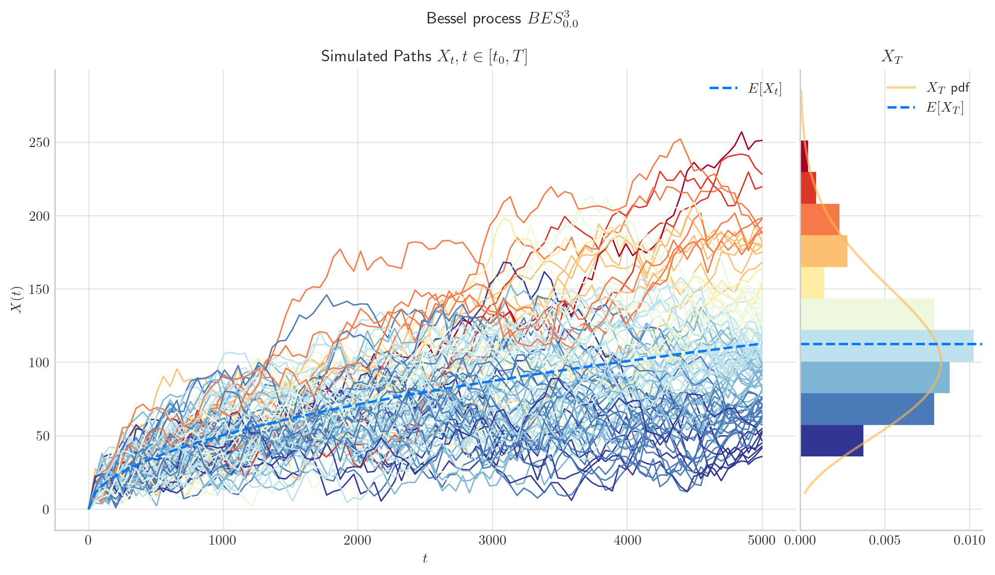
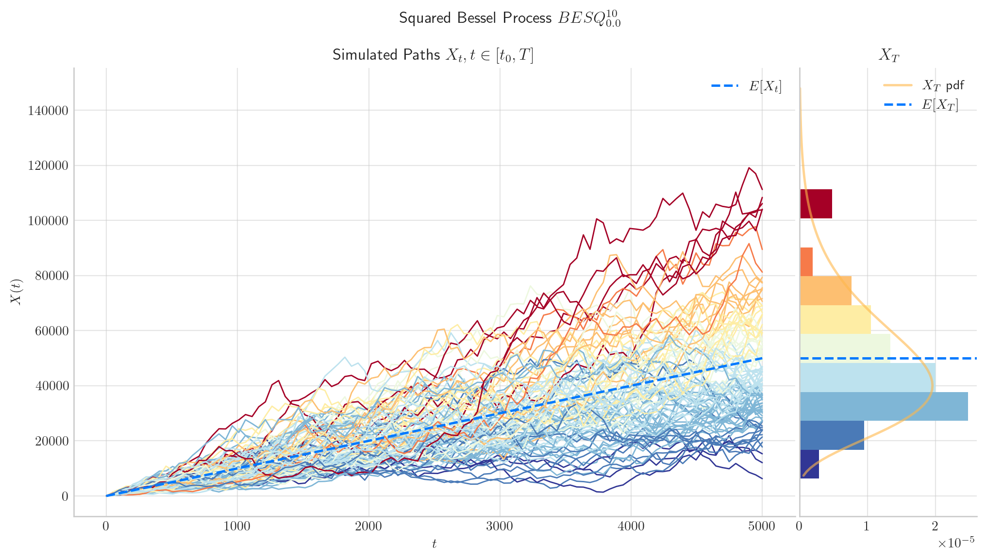
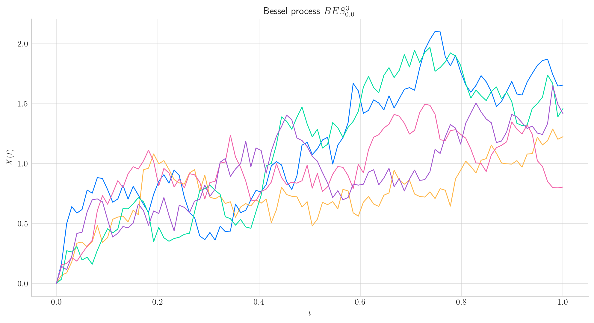
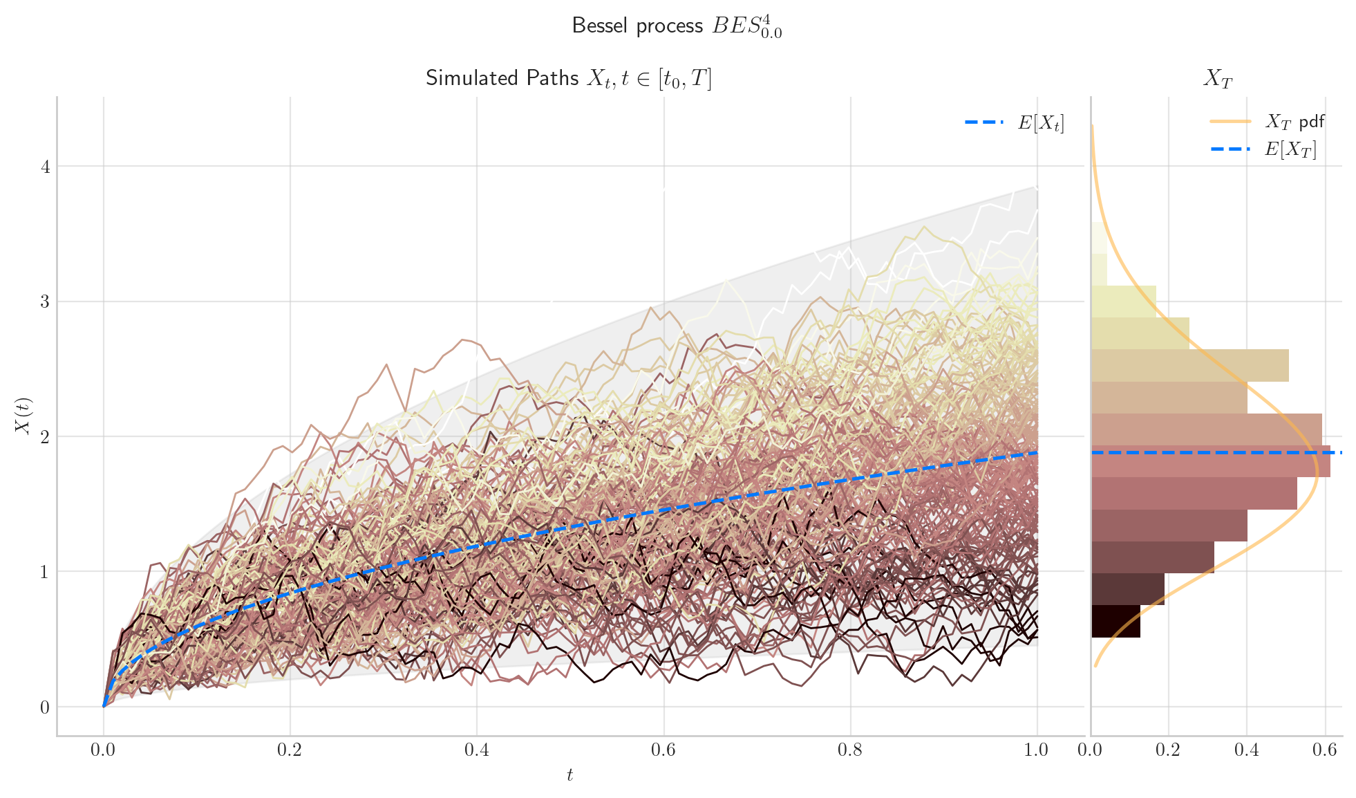
6.5. Final Visualisations

To finish this note, let us take a look at some simulations.

# from aleatory.processes import BESProcess
bes = BESProcess(dim=4, T=1)
fig = bes.draw(n=100, N=200, envelope=True, colormap="pink", figsize=(12,6))

# from aleatory.processes import BESQProcess
bes = BESQProcess(dim=6, T=1.0)
fig = bes.draw(n=100, N=200, envelope=True, colormap="cool")

# from aleatory.processes import BESProcess
# import matplotlib.pyplot as plt
# import numpy as np

process = BESProcess(dim=2, T=10, rng=np.random.default_rng(seed=1234))
paths = process.simulate(n=1000, N=4)
ts = process.times
exp = process.marginal_expectation(ts)

for path in paths:
    plt.plot(ts, path)
plt.plot(ts, exp, color='grey',linewidth=2, label=f'$E[X_t]$')
plt.legend()
plt.title('Four Paths from a Bessel Process\n' + process.name)
plt.show()

# from aleatory.processes import BESQProcess
# import matplotlib.pyplot as plt
# import numpy as np

process = BESQProcess(dim=2, T=10, rng=np.random.default_rng(seed=12345))
paths = process.simulate(n=1000, N=4)
ts = process.times
exp = process.marginal_expectation(ts)

for path in paths:
    plt.plot(ts, path)
plt.plot(ts, exp, color='grey',linewidth=2, label=f'$E[Y_t]$')
plt.legend()
plt.title('Four Paths from a Squared Bessel Process\n' + process.name)
plt.show()

6.6. References and Further Reading

• “Mathematical Methods for Financial Markets” by Monique Jeanblanc, Marc Yor, Marc Chesney; Springer Science & Business Media, 13 Oct 2009

• Notes on Bessel Processes by Gregory F. Lawler

• A Survey and Some Generalizations of Bessel Processes by Anja Göing-Jaeschke and Marc Yor; Bernoulli Vol. 9, No. 2 (Apr., 2003), pp. 313-349 (37 pages)

• Squared Bessel processes of positive and negative dimension embedded in Brownian local times by Jim Pitman, Matthias Winkel; Electron. Commun. Probab. 23: 1-13 (2018). DOI: 10.1214/18-ECP174