2. Brownian Motion with Drift

The purpose of this notebook is to review and illustrate the Brownian motion with Drift, also called Arithmetic Brownian Motion, and some of its main properties.

Before diving into the theory, let’s start by loading the libraries

• matplotlib

• aleatory

together with the style sheet Quant-Pastel Light.

These tools will help us to make insightful visualisations.

import matplotlib.pyplot as plt
mystyle = "https://raw.githubusercontent.com/quantgirluk/matplotlib-stylesheets/main/quant-pastel-light.mplstyle"
plt.style.use(mystyle)
plt.rcParams["figure.figsize"] = (12, 6)

from aleatory.processes import BrownianMotion
process = BrownianMotion(drift=1.0, scale=0.50)
process.draw(n=200, N=200, envelope=True, title=f"Arithmetic Browniam Motion")
plt.show()

2.1. Definition

The Arithmetic Brownian motion can be defined by the following Stochastic Differential Equation (SDE)

(2.1)\[\begin{equation} dX_t = \mu dt + \sigma dW_t, \quad t >0, \end{equation}\]

with initial condition \(X_0 =x_0\), and constant parameters \(\mu\in \mathbb{R}\), \(\sigma>0\). Without loss of generality we are going to assume that \(x_0=0\). Here, \(W_t\) denotes a standard Brownian motion.

Equation (2.1) equivales to

(2.2)\[\begin{align} X_t &= \int_0^t \mu ds + \int_0^t \sigma dW_t = \mu t + \sigma W_t, \end{align}\]

which gives us the solution.

2.2. Marginal Distributions

The las equation implies that for each \(t>0\), the marginal \(X_t|X_0\) (which we will denote by \(X_t\) for simplicity) is normally distributed since it is the sum of a deterministic part plus the marginal of a standard Brownian motion \(W_t\) –which follows a Gaussian distritbuion \(\mathcal{N}(0,t)\) times a constant .

2.2.1. Expectation, Variance, and Covariance

From equation (2.2) we obtain

\[\begin{equation*} \mathbf{E} [X_t] = E [X_t |X_0] = \mu t, \qquad \forall t\geq 0, \end{equation*}\]

and

\[\begin{equation*} \mathbf{Var} [X_t] = Var[X_t |X_0] = \sigma^2 t, \qquad \forall t> 0. \end{equation*}\]

So we have

(2.3)\[\begin{equation} X_t \sim \mathcal{N}(\mu t, \sigma^2 t), \qquad \forall t>0. \end{equation}\]

Besides, for any \( t > s >0\), we have

\[\begin{align*} \mathbf{Cov} [X_t, X_s] &= \sigma^2 \min\{s, t\},\\ \end{align*}\]

using the properties of the covariance and the fact that

\[\begin{equation*} \mathbf{Cov} [W_t, W_s] = \min\{s, t\}, \qquad \forall s, t>0. \end{equation*}\]

2.2.2. Marginal Distributions in Python

Equation (2.3) allows us to implement the marginal distributions with Python.

One way to do this is by using the object norm from the library scipy.stats.

The next cell shows how to create \(X_1\) using this method.

import numpy as np
from scipy.stats import norm
mu = 1.0
sigma = 0.25
t = 1.0

X_1 = norm(loc=mu*t, scale= sigma*np.sqrt(t))

Now, we can call the method stats to obtain the mean, variance, skewness, and kurtosis of the distribution.

X_1.stats(moments='mvsk')

(array(1.), array(0.0625), array(0.), array(0.))

Another way to do this is by creating an object BrownianMotion from aleatory.processes and calling the method get_marginal on it.

The next cell shows how to create the marginal \(X_1\) using this method. Just as before, we call the method stats to obtain the mean, variance, skewness, and kurtosis of the distribution.

from aleatory.processes import BrownianMotion
process = BrownianMotion(drift=1.0, scale=0.25)
X_1 = process.get_marginal(t=1)

X_1.stats(moments='mvsk')

(array(1.), array(0.0625), array(0.), array(0.))

Hereafter, we will use the latter method to create marginal distributions from the arithmetic Brownian Motion.

2.2.3. Probability Density Functions

The probability density function (pdf) of the marginal distribution \(X_t|X_0\) is given by the following expression

\[\begin{equation*} f(x, t; \mu, \sigma) = \dfrac{1}{\sigma \sqrt{2 \pi t}}\exp\left\{ -\dfrac{1}{2} \left(\dfrac{x-\mu t}{\sigma \sqrt{t}}\right)^2 \right\}, \qquad \forall x\in\mathbb{R}, t>0. \end{equation*}\]

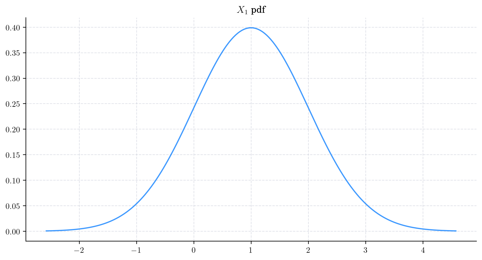
2.2.3.1. Visualisation

In order to visualise these functions, we are going to load the library matplotlib and set some formatting options.

import matplotlib.pyplot as plt

plt.style.use("seaborn-v0_8-whitegrid")
plt.rcParams["figure.figsize"] = (12, 6)
%config InlineBackend.figure_format ='retina'

Now, we consider an arithmetic Brownian Motion BrownianMotion(drift=1.0, scale=1.0) and plot the probability density function of \(X_1\) as follows.

process = BrownianMotion(drift=1.0, scale=1.0)
X_1 = process.get_marginal(t=1)
x = np.linspace(X_1.ppf(0.005) -1 , X_1.ppf(0.995)+1,200)
plt.plot(x, X_1.pdf(x), '-', lw=1.5, alpha=0.75, label=f'$t$={1:.2f}')
plt.title(f'$X_1$ pdf')
plt.show()

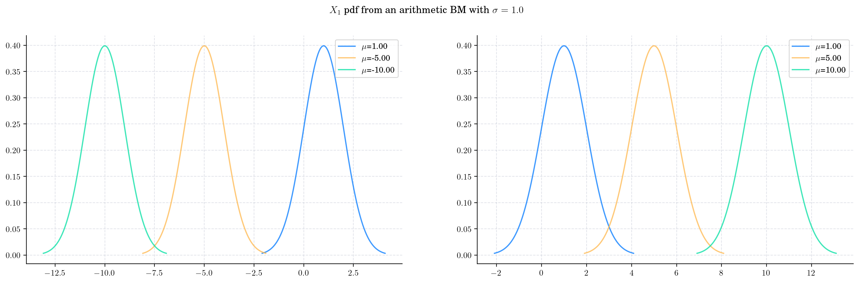
Next, we vary the value of the parameter \(\mu\) and plot the corresponding pdfs. Clearly, the mean of the distribution moves along with \(\mu\) (in this case it is equal to \(\mu\) since \(t=1\)) while the variance stays the same.

fig, axs = plt.subplots(1, 2, figsize=(18, 6))
mu_values = ([1,  -5.0, -10], [1,5 , 10])
for (mus, ax) in zip(mu_values, axs):
    for mu in mus:
        process = BrownianMotion(drift=mu, scale=1.0)
        X_t = process.get_marginal(t=1.0)
        x = np.linspace(X_t.ppf(0.001), X_t.ppf(0.999), 100)
        ax.plot(x, X_t.pdf(x), '-', lw=1.5,
                alpha=0.75, label=f'$\mu$={mu:.2f}')
        ax.legend()
fig.suptitle(r'$X_1$ pdf from an arithmetic BM  with $\sigma=1.0$')
plt.show()

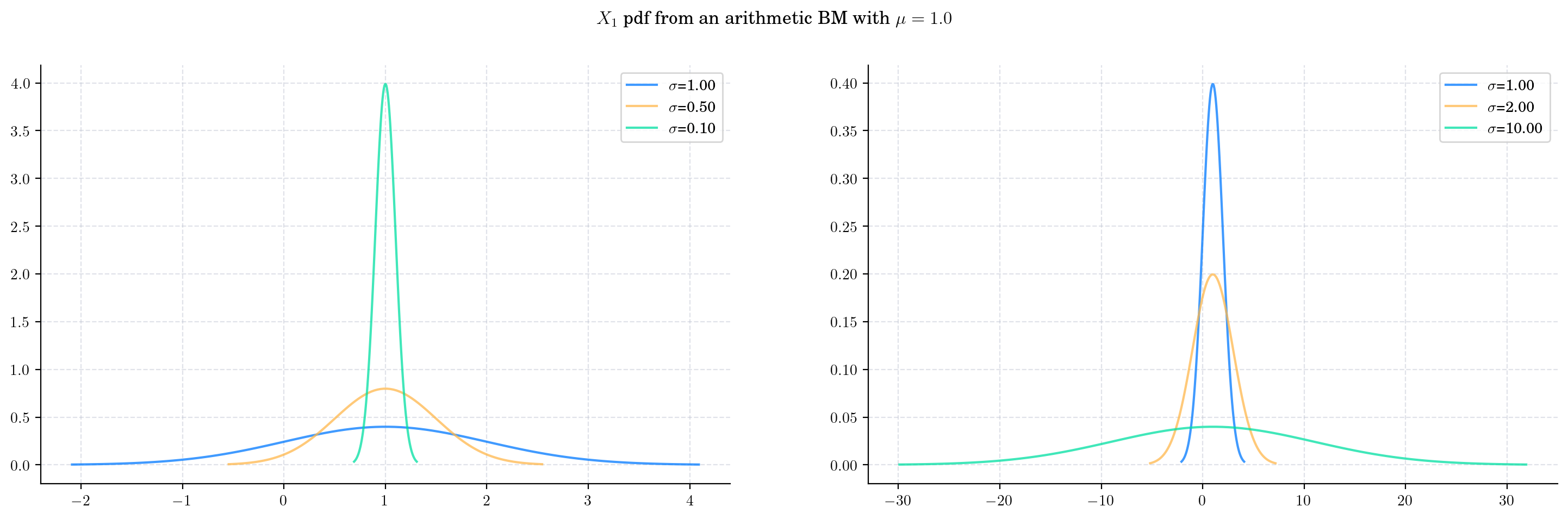
Similarly, we vary the value of the parameter \(\sigma\) and plot the corresponding pdfs. This time, the mean of the distribution remains contant while the variance moves along with the value of \(\sigma\). As \(\sigma\) grows, the density becomes wider.

fig, axs = plt.subplots(1, 2, figsize=(18, 6))
sigma_values = ([1,  0.5, 0.1], [1, 2, 10])
for (sigmas, ax) in zip(sigma_values, axs):
    for sigma in sigmas:
        process = BrownianMotion(drift=1.0, scale=sigma)
        X_t = process.get_marginal(t=1.0)
        x = np.linspace(X_t.ppf(0.001), X_t.ppf(0.999), 100)
        ax.plot(x, X_t.pdf(x), '-', lw=1.5,
                alpha=0.75, label=f'$\sigma$={sigma:.2f}')
        ax.legend()
fig.suptitle(r'$X_1$ pdf from an arithmetic BM  with $\mu=1.0$')
plt.show()

Finally, let’s see what happens when we keep the parameters constant but \(t\) grows. For this, we will consider two cases, \(\mu>0\) and \(\mu<0\).

for mu in [1.0, -1.0]:
    process = BrownianMotion(drift=mu, scale=1.)
    fig, ax1 = plt.subplots(1, 1)
    for t in [1,5, 10]:
        X_t= process.get_marginal(t)
        x = np.linspace(X_t.ppf(0.001), X_t.ppf(0.999), 100)
        ax1.plot(x, X_t.pdf(x), '-', lw=1.5,
                alpha=0.75, label=f'$t$={t:.2f}')
    ax1.legend()
    plt.title(f'$X_t$ pdfs from an arithmetic BM with $\mu$={mu} and $\sigma$={1.0}')
    plt.show()

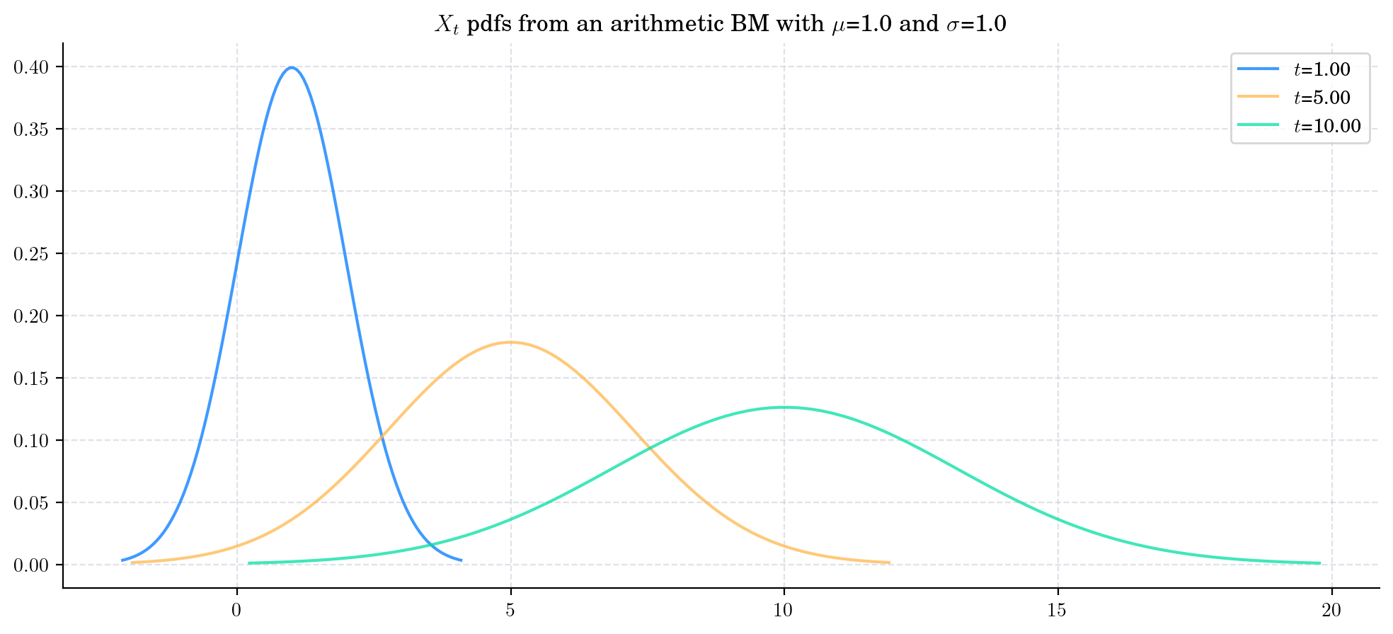
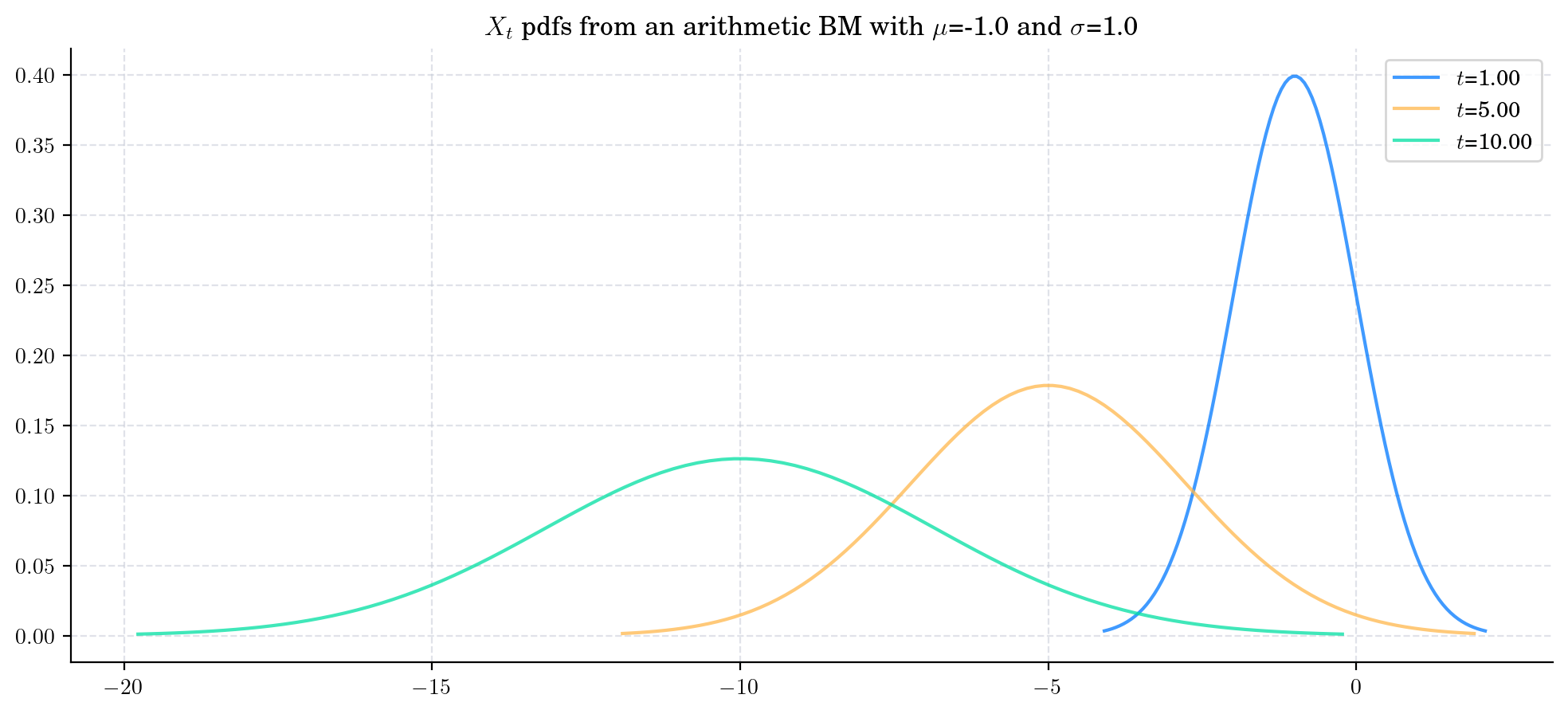
In these charts, we can see the characteristic symmetric bell-shaped curves of the normal/Gaussian distribution. Moreover, we can make the following observations:

• \(X_t\) will clearly take positive and negative values

• If the drift is positive/negative, then \(X_t\) will take bigger/smaller (in magnitude) values more likely as \(t\) increases

• If the drift is positive/negative, then the pdfs of \(X_t\) moves towards the right/left as \(t\) increases.

• The pdfs of \(X_t\) flatten/spread as \(t\) increases.

2.2.4. Sampling

Now, let’s see how to obtain a random sample from the marginal \(X_t\) for \(t>0\).

The next cell shows how to get a sample of size 5 from \(X_1\).

from aleatory.processes import BrownianMotion
process = BrownianMotion(drift=1.0, scale=0.25)
X_t = process.get_marginal(t=1.0) 
X_t.rvs(size=5)

array([0.48557417, 0.8879651 , 0.89372702, 1.53927062, 1.24491245])

2.3. Simulation

In order to simulate paths from a stochastic process, we need to set a discrete partition over an interval for the simulation to take place.

For simplicity, we are going to consider an equidistant partition of size \(n\) over \([0,T]\), i.e.:

\[\begin{equation*} t_i = \frac{i}{n-1} T \qquad \hbox{for } i = 0, \cdots, n-1. \end{equation*}\]

Then, the goal is to simulate a path of the form \(\{ X_{t_i} , i=0,\cdots, n-1\}\). There are a number of ways to do this. Here, we are going to use equation (2), i.e.

\[\begin{equation*} X_t = \mu t + \sigma W_t, \end{equation*}\]

and the fact that we know how to simulate a Brownian Motion (see Brownian Motion for details).

First, we construct the partition, using np.linspace, and calculate the standard deviation of the normal random variable \(\mathcal{N}(0, \frac{T}{n-1})\), i.e.:

\[\sigma = \sqrt{\frac{T}{n-1}}.\]

from aleatory.processes import BrownianMotion

T = 1.0
n = 100
mu = 1.0
sigma = 0.25
t = 1.0
times = np.linspace(0, T, n)  # Partition
BM = BrownianMotion(T=T)
bm_path = BM.sample_at(times)
abm_path = mu*times + sigma*bm_path

Next, we calculate the normal increments and take to cumulative sum.

Note

Note that we add the initial point of the Brownian motion, i.e. \(W_0 = 0\).

normal_increments = norm.rvs(loc=0, scale=sigma, size=n-1) # Sample of size n-1
normal_increments = np.insert(normal_increments, 0, 0) # This is the initial point
Wt = normal_increments.cumsum() # Taking the cumulative sum

Now, let’s plot our simulated path!

plt.plot(times, abm_path, 'o-', lw=1)
plt.title('Arithmetic Brownian Motion Path')
plt.show()

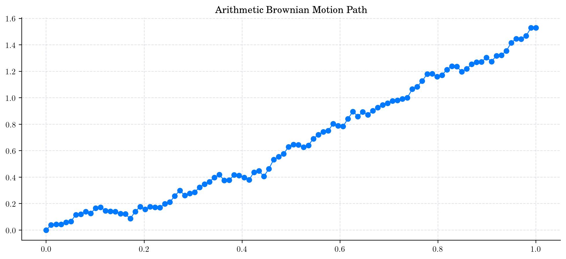
Note

In this plot, we are using a linear interpolation to draw the lines between the simulated points.

2.3.1. Simulating and Visualising Paths

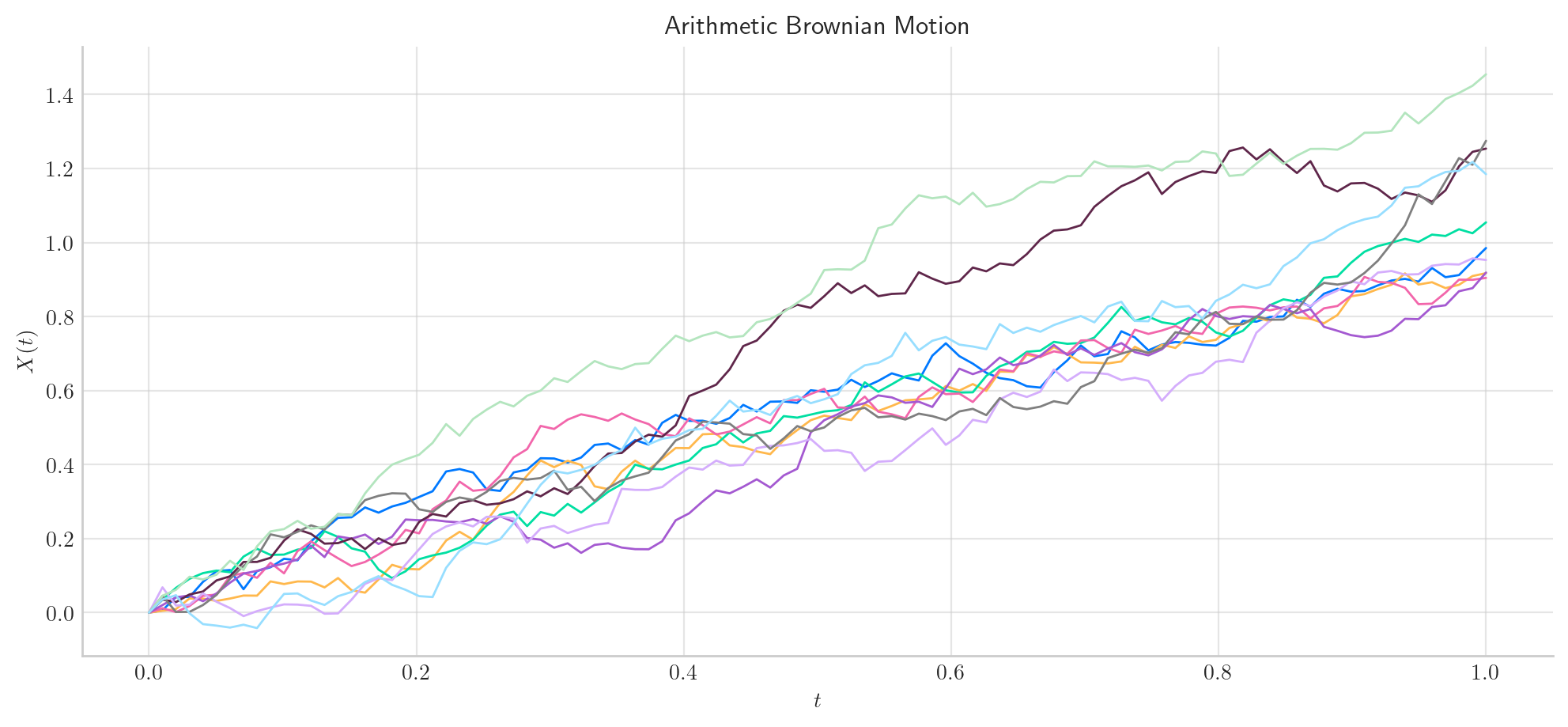
To simulate several paths from an Arithmetic Brownian Motion and visualise them we can use the method plot from the aleatory library.

Let’s simulate 10 paths over the interval \([0,1]\) using a partition of 100 points.

Tip

Remember that the number of points in the partition is defined by the parameter \(n\), while the number of paths is determined by \(N\).

process = BrownianMotion(drift=1.0, scale=0.25)
process.plot(n=100, N=10)
plt.show()

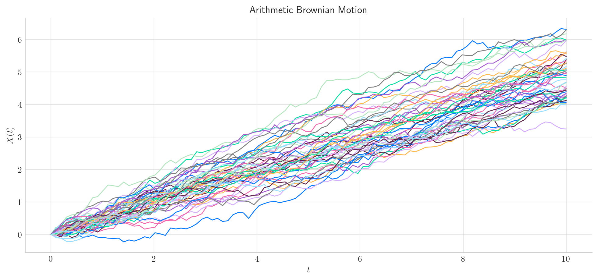
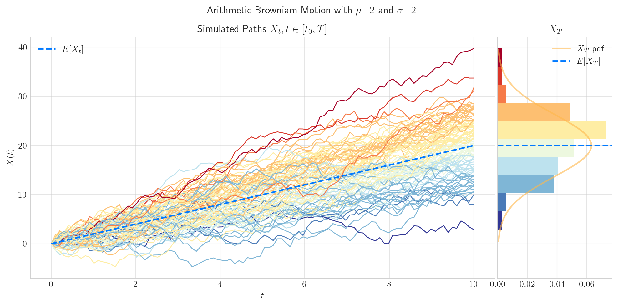
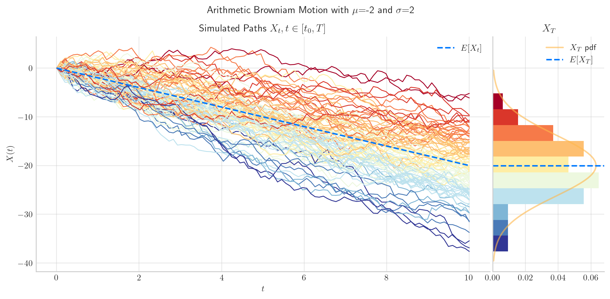
Similarly, we can define an arithmetic Brownian Motion over the interval \([0, 10]\) and simulate 50 paths with a partition of size 100.

process = BrownianMotion(drift=0.5, scale=0.25, T=10)
process.plot(n=100, N=50)
plt.show()

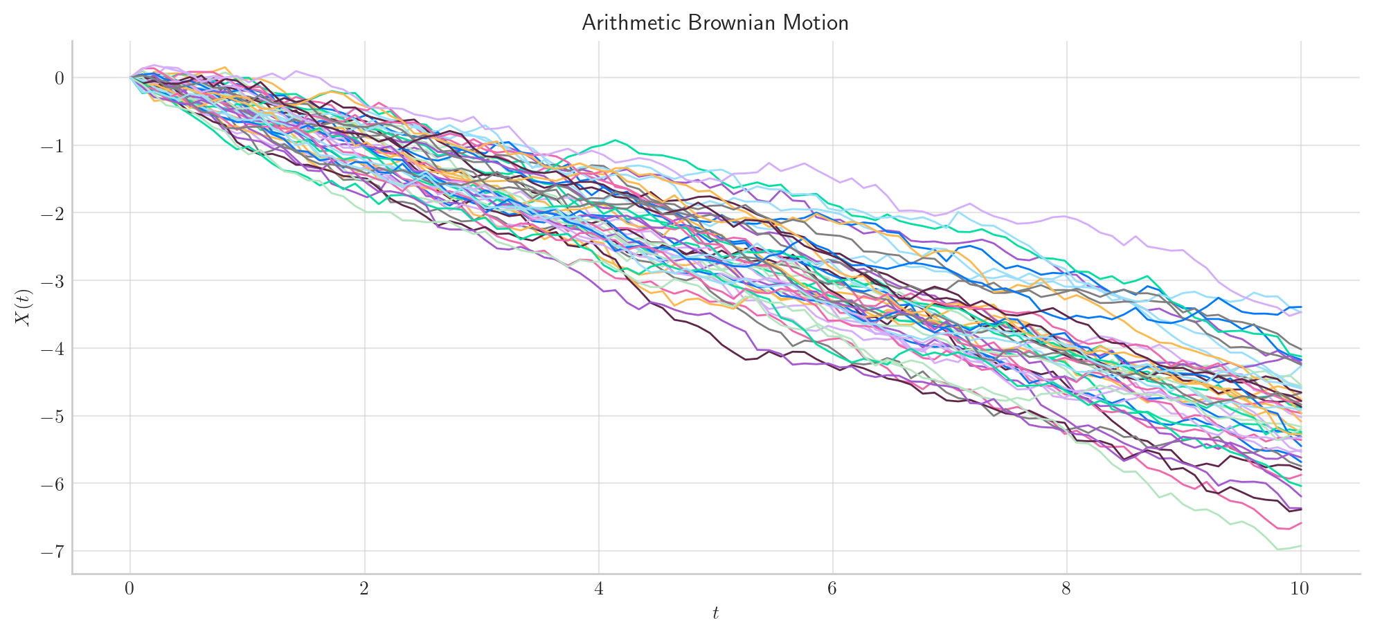
process = BrownianMotion(drift=-0.5, scale=0.25, T=10)
process.plot(n=100, N=50)
plt.show()

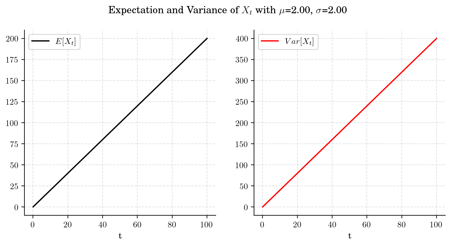
2.4. Long Time Behaviour

2.4.1. Expectation and Variance

We have

\[\begin{equation*} \lim_{t\rightarrow\infty} \mathbf{E}\left[X_t \right] = \lim_{t\rightarrow\infty} \mu t = \begin{cases} \infty, \hbox{ if } \mu>0\\ 0 \hbox{ if } \mu=0\\ -\infty, \hbox{ if } \mu<0, \\ \end{cases} \end{equation*}\]

and

\[\begin{equation*} \lim_{t\rightarrow\infty}\mathbf{Var}[ X_t] = \lim_{t\rightarrow\infty} \sigma^2 t = \infty. \end{equation*}\]

Next, we illustrate the convergence of both the mean and the variance as \(t\) grows under the two cases \(\mu>0\) and \(\mu<0\) (\(\mu=0\) is trivial).

def draw_mean_variance(mu, sigma, T=100):

    process = BrownianMotion(drift=mu, scale=sigma, T=T)
    ts = np.linspace(0.1, T, T)
    means = process.marginal_expectation(ts)
    variances = process.marginal_variance(ts)
    fig, (ax1, ax2,) = plt.subplots(1, 2, figsize=(9, 4))
    
    ax1.plot(ts, means, lw=1.5, color='black', label='$E[X_t]$')
    ax1.set_xlabel('t')
    ax1.legend()
    ax2.plot(ts,  variances, lw=1.5, color='red', label='$Var[X_t]$')
    ax2.set_xlabel('t')
    ax2.legend()
    fig.suptitle(
        'Expectation and Variance of $X_t$ with ' f'$\mu$={mu:.2f}, $\sigma$={sigma:.2f}', size=12)
    plt.show()

draw_mean_variance(mu=2., sigma=2., T=100)

draw_mean_variance(mu=-2., sigma=2., T=100)

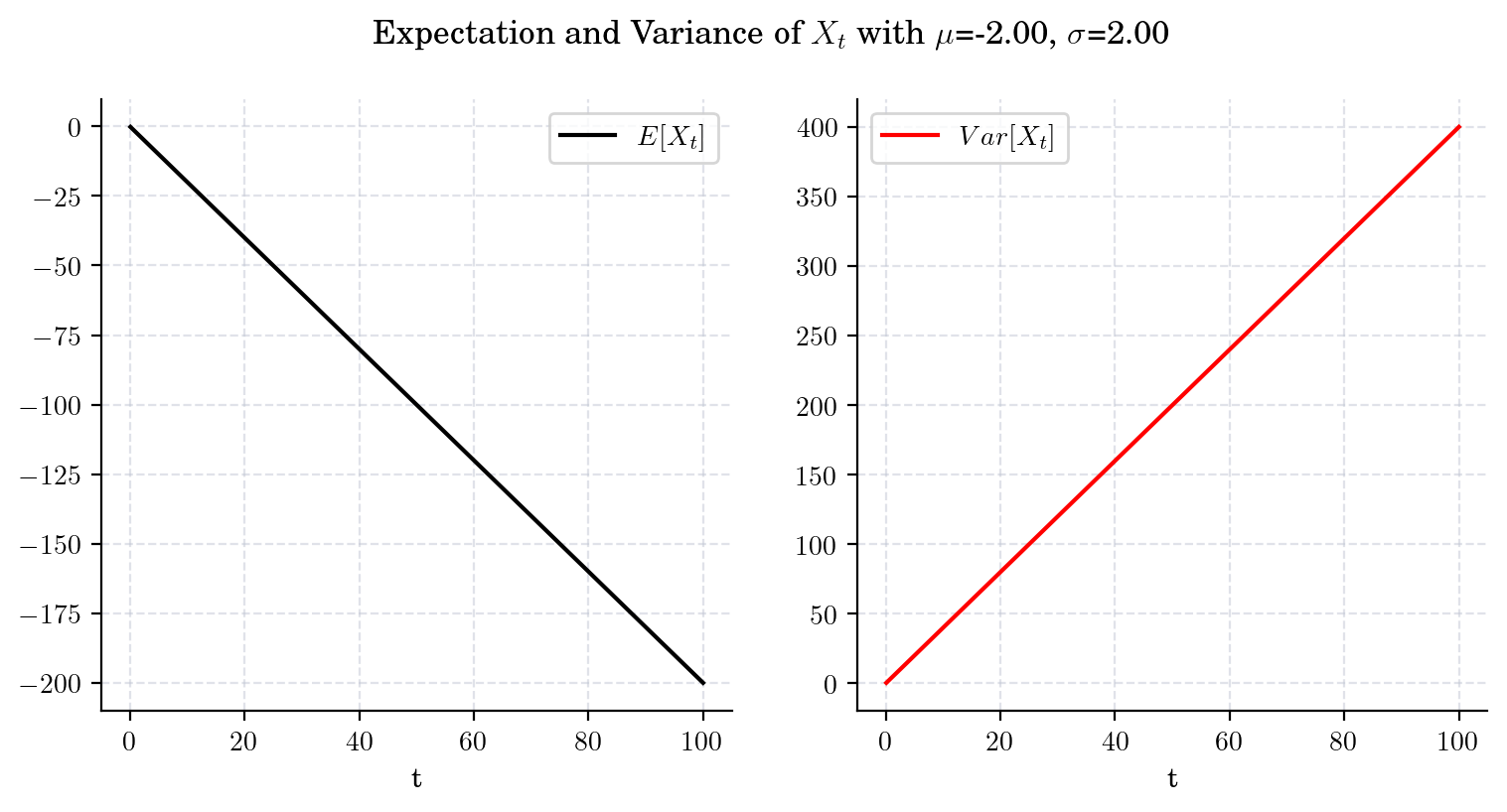
Finally, let’s take a look at how the process simulations look under these two cases.

process = BrownianMotion(drift=2.0, scale=2.0, T=10)
process.draw(n=100, N=100, title=f"Arithmetic Browniam Motion with $\mu$=2 and $\sigma$=2")
plt.show()

process = BrownianMotion(drift=-2.0, scale=2.0, T=10)
process.draw(n=100, N=100, title=f"Arithmetic Browniam Motion with $\mu$=-2 and $\sigma$=2")
plt.show()

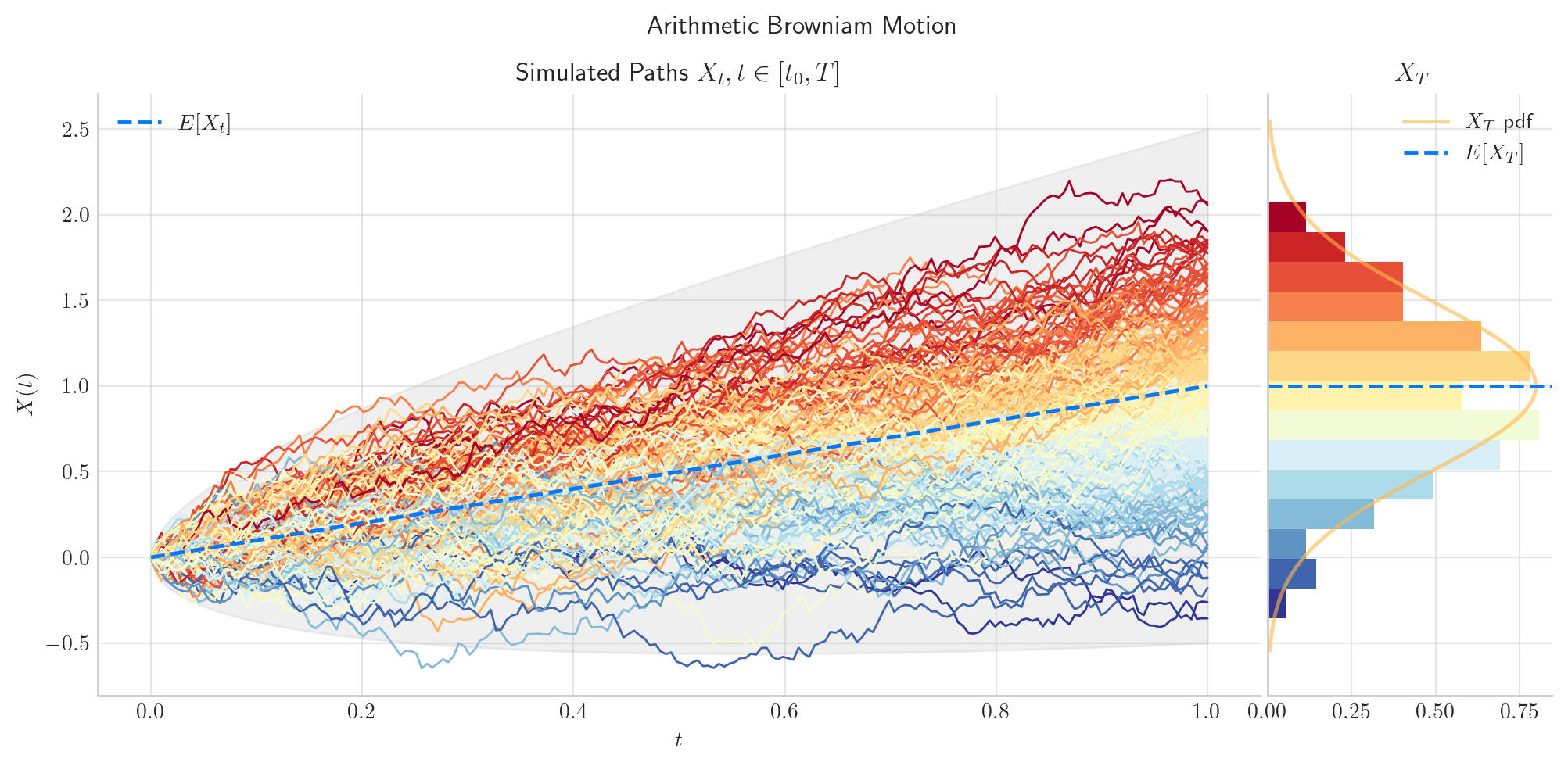
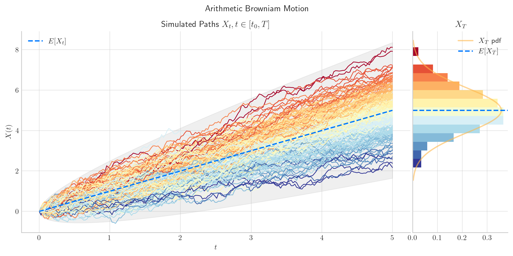
2.5. Visualisation

To finish this note, let’s take a final look at a simulation from the arithmetic Brownian Motion.

from aleatory.processes import BrownianMotion
process = BrownianMotion(drift=1.0, scale=0.50, T=5.0)
process.draw(n=200, N=200, envelope=True, title=f"Arithmetic Browniam Motion")
plt.show()

2.6. References and Further Reading

• Brownian Motion Notes by Peter Morters and Yuval Peres (2008).