8. Bessel Processes Part III#
The purpose of these notebooks (Bessel Processes Part I-III) is to provide an illustration of the Bessel Processes and some of their main properties.
In Part I, we introduce both Bessel and Squared Bessel processes with integer dimension \(d\geq 2,\) and study some of its main properties.
In Part II, we show that Bessel processes with integer dimension satisfy certain Stochastic Differential Equations (SDEs). This representation allows us to extend them to the non-integer case.
Finally, in Part III we illustrate both Bessel and Squared Bessel processes with general dimension \(\delta \geq 0\), and some of its main properties.
Before diving into the theory, let’s start by loading the following libraries
matplotlib
together with the style sheet Quant-Pastel Light.
from aleatory.processes import BESProcess, BESQProcess
import matplotlib.pyplot as plt
mystyle = "https://raw.githubusercontent.com/quantgirluk/matplotlib-stylesheets/main/quant-pastel-light.mplstyle"
plt.style.use(mystyle)
plt.rcParams["figure.figsize"] = (12,6)
These tools will help us to make insightful visualisations of Bessel processes.
8.1. Definition#
For every \(\delta\geq 0\) and \(x\geq 0\), a Bessel process with dimension \(\delta\) started at \(x\) is defined as the unique strong solution of the SDE
and is denoted by \(BES^{\delta}_{x}\).
For every \(\delta\geq 0\) and \(y\geq 0\), a Squared Bessel process with dimension \(\delta\) started at \(y\) is defined as the unique strong solution of the SDE
and is denoted by \(BESQ^{\delta}_y\).
Bessel processes are frequently parameterised in terms of the quantity
which is called index of the process.
Notation
Hereafter, we will use the following notation:
\(BES^{\delta}_x\) or \(BES^{(\nu)}_x\) : to denote a Bessel process of dimension \(\delta\) started at \(x\)
\(BESQ^{\delta}_y\) or \(BESQ^{(\nu)}_y\): to denote a Squared Bessel process of dimension \(\delta\) started at \(y\).
8.1.1. Transition Densities#
For any \(\delta >0\) (or equivalently \(\nu>-1\)) the transition density \(p_t^{(\nu)}\) of a Bessel process \(BES^{(\nu)}\) is given by
and the transition density \(q_t^{(\nu)}\) of a Squared Bessel process \(BESQ^{(\nu)}\) is given by
where \(I_{\nu}\) is the usual modified Bessel function with index \(\nu\).
Note that
8.2. Marginal Distributions#
The definition of the transition densities imply the following about the marginal distributions.
Given a Bessel process \(X \sim BES_x^{(\nu)}\) the marginal distribution \(X_t|X_0\) (denoted as \(X_t\) for simplicity) has density function
Thus, the marginal is a scaled non-central Chi random variable with \(\delta\) degrees of freedom and non-centrality parameter \(\frac{x}{\sqrt{t}}\), i.e.:
Given a Squared Bessel process \(Y\sim BESQ_y^{(\nu)}\) the marginal distribution \(Y_t|Y_0\) (denoted as \(Y_t\) for simplicity) has density function
Thus the marginal is a scaled non-central Chi squared random variable with \(\delta\) degrees of freedom and non-centrality parameter \(\frac{y}{t}\), i.e.:
Note
The number of degrees of freedom does not depend on \(t\), which means that the number of degrees of freedom remains constant as the process evolves.
The non-centrality parameter tends to zero as \(t\) grows.
8.2.1. Visualisation#
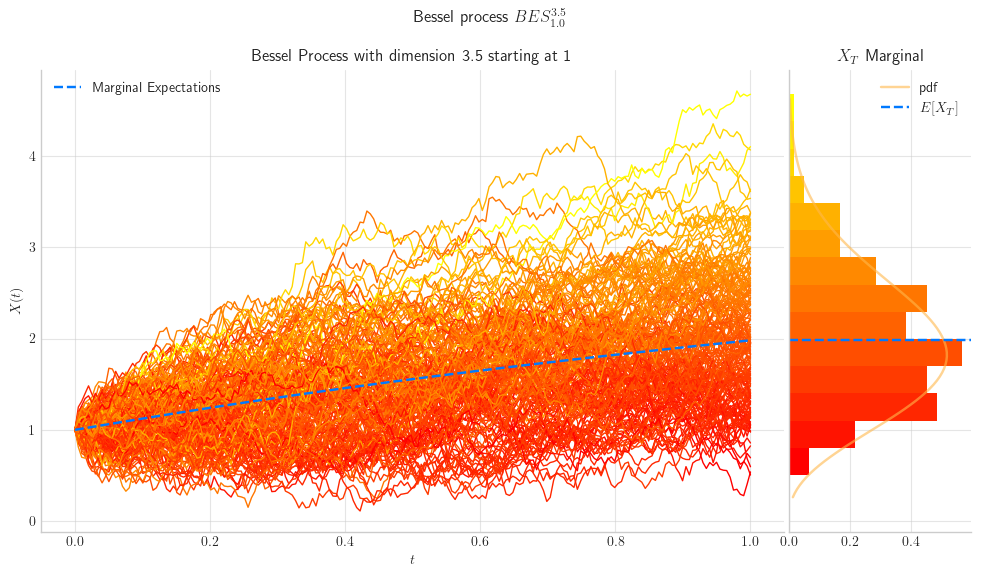
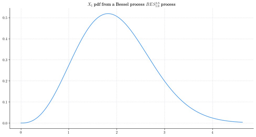
To visualise these probability density functions in Python, we can use the method get_marginal from the aleatory library. Let’s consider a Bessel process BESProcess(dim=3.5, initial=1.0) and plot the density function of the marginal \(X_1\)
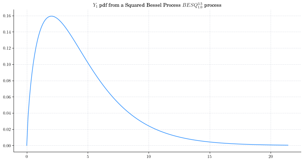
Similarly, we can take a Squared Bessel process BESQProcess(dim=3.5, initial=1.0) and plot the density function of \(Y_1\).
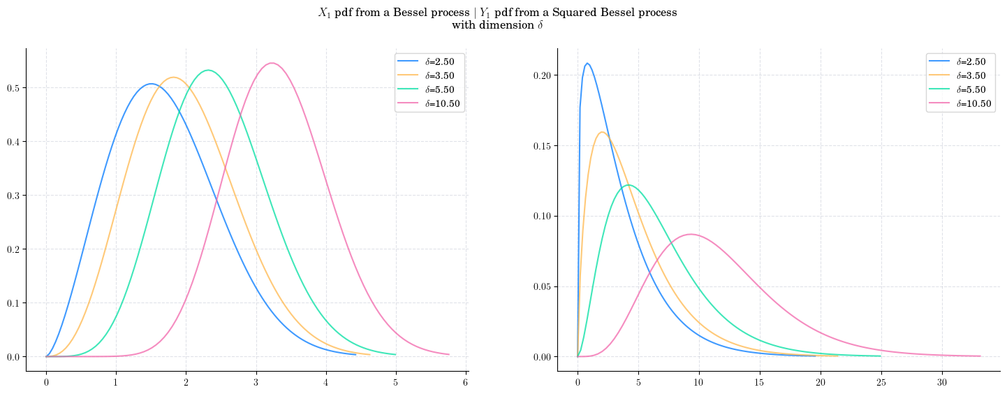
Next, we vary the value of the dimension \(\delta\) and plot the corresponding pdfs. As the dimension increases:
The density from the Bessel marginal moves towards the right and becomes more symmetric.
The density from the Squared Bessel marginal also move towards the right, it becomes wider and its shape changes as well.
<>:8: SyntaxWarning: invalid escape sequence '\d'
<>:10: SyntaxWarning: invalid escape sequence '\m'
<>:8: SyntaxWarning: invalid escape sequence '\d'
<>:10: SyntaxWarning: invalid escape sequence '\m'
/var/folders/8_/ln4xq0tn2_9dclcldppw87f00000gn/T/ipykernel_65058/20272281.py:8: SyntaxWarning: invalid escape sequence '\d'
  ax.plot(x, X_t.pdf(x), '-', lw=1.5, alpha=0.75, label=f'$\delta$={d:.2f}')
/var/folders/8_/ln4xq0tn2_9dclcldppw87f00000gn/T/ipykernel_65058/20272281.py:10: SyntaxWarning: invalid escape sequence '\m'
  fig.suptitle(f'$X_1$ pdf from a Bessel process $\mid$  $Y_1$ pdf from a Squared Bessel process\n with dimension $\delta$')
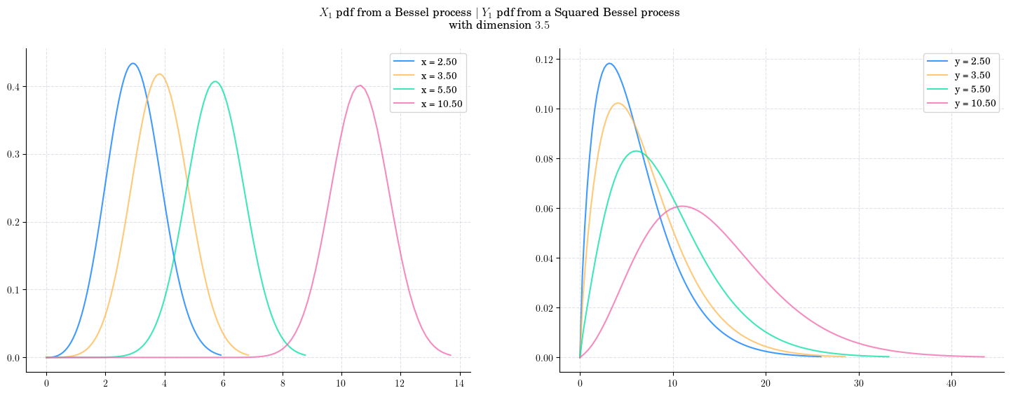
Now, we fix the dimension to \(\delta =3.5\) vary the value of the initial condition and plot the corresponding pdfs. As the initial condition increases:
The density from the Bessel marginal moves towards the right and becomes less leptokurtic
The density from the Squared Bessel margina becomes wider and more symmetric.
<>:11: SyntaxWarning: invalid escape sequence '\m'
<>:11: SyntaxWarning: invalid escape sequence '\m'
/var/folders/8_/ln4xq0tn2_9dclcldppw87f00000gn/T/ipykernel_65058/2623012637.py:11: SyntaxWarning: invalid escape sequence '\m'
  fig.suptitle(f'$X_1$ pdf from a Bessel process $\mid$  $Y_1$ pdf from a Squared Bessel process\n with dimension $3.5$')
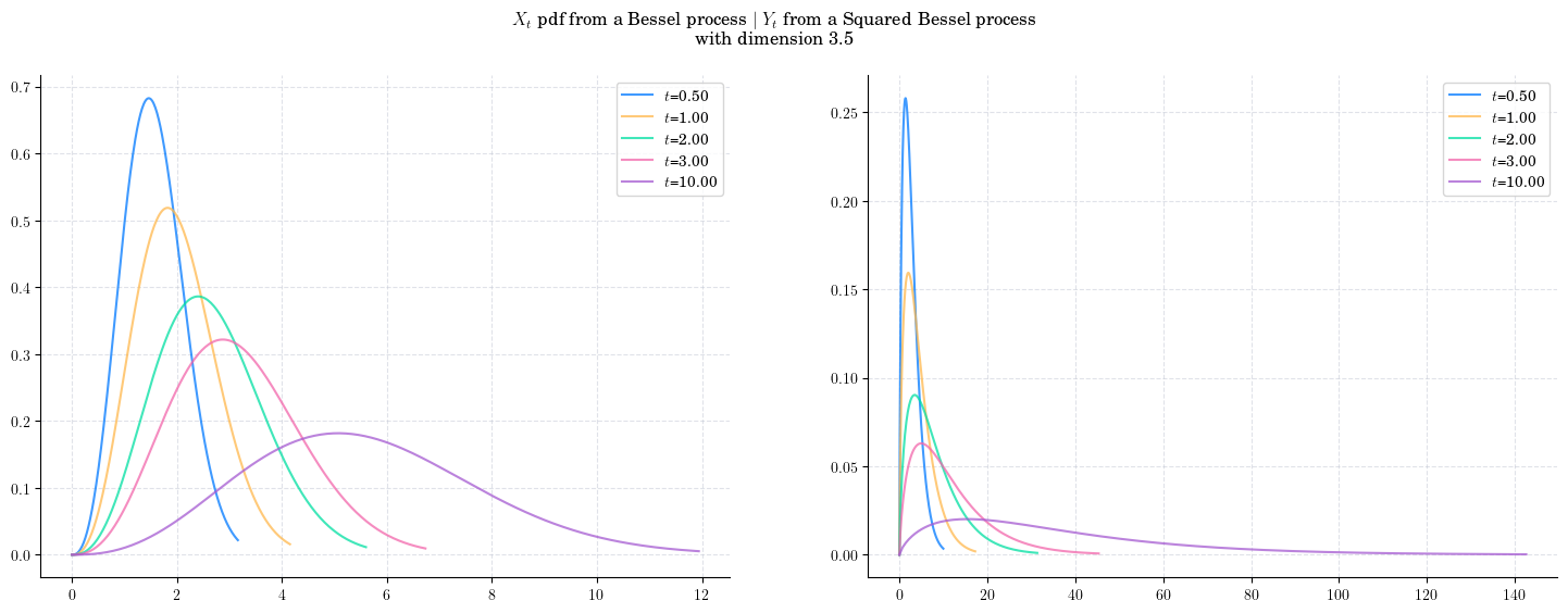
Finally, we fix both the dimension and the initial condition and vary the value of time \(t\) and plot the corresponding pdfs. As \(t\) increases:
The density from the Bessel marginal moves towards the right and becomes wider.
The density from the Squared Bessel marginal becomes wider very rapidly as \(t\) grows.
<>:14: SyntaxWarning: invalid escape sequence '\m'
<>:14: SyntaxWarning: invalid escape sequence '\m'
/var/folders/8_/ln4xq0tn2_9dclcldppw87f00000gn/T/ipykernel_65058/1596705777.py:14: SyntaxWarning: invalid escape sequence '\m'
  fig.suptitle(f'$X_t$ pdf from a Bessel process $\mid$ $Y_t$ from a Squared Bessel process\n with dimension 3.5')
8.2.2. Expectation and Variance#
8.2.2.1. Bessel#
For each \(t>0\), the marginal distribution \(X_t|X_0=x\) from a Bessel process \(BES_x^{\delta}\) satisfies
where \(L_{\frac{1}{2}}^{\nu}\) denotes the generalised Laguerre polynomial; and
where \(\mu = \mathbf{E}[X_t]\).
Clearly, the expression for the variance coincide with the one from Bessel Processes Part I when \(x=0\) and \(\delta\) is integer. To see that the same is true for the expectation, one should note that the Laguerre polynomials satisfy
8.2.2.1.1. Python Implementation#
We can use the method get_marginal to obtain the marginal distribution and the get its mean and variance
from aleatory.processes import BESProcess
delta = 3.5
x = 1.0
t = 2
bes = BESProcess(dim=delta, initial=x)
marginal = bes.get_marginal(t=t)
print(marginal.mean())
print(marginal.var())
2.6378008359694296
1.0420067497589793
8.2.2.2. Squared Bessel#
For each \(t>0\), the conditional marginal \(Y_t|Y_0=y\) from a Squared Bessel process \(BESQ_y^{\delta}\) satisfies
and
Clearly, these expressions coincide with the ones from Bessel Processes Part I when \(x=0\) and \(\delta\) is integer.
8.2.2.2.1. Python Implementation#
For given \(\delta, y, t\geq 0\), we can implement the above formulas for the expectation, and variance, as follows.
delta = 3.5
y = 1.0
t= 2.0

expectation = t*(delta + y/t)
variance = (2.0*t**2)*(delta + 2.0*y/t)

print(f'For d={d}' , f't={t}', sep=", ")
print(f'E[X_t] = {expectation: .6f}')
print(f'Var[X_t] = {variance :.6f}')
For d=3.5, t=2.0
E[X_t] =  8.000000
Var[X_t] = 36.000000
We can also use the method get_marginal to obtain the marginal distribution and the get its mean and variance
# from aleatory.processes import BESProcess
delta = 3.5
y = 1.0
t = 2.0
bes = BESQProcess(dim=delta, initial=y)
marginal = bes.get_marginal(t=t)
print(marginal.mean())
print(marginal.var())
8.0
36.0
8.3. Long Time Behaviour#
8.3.1. Expectation and Variance#
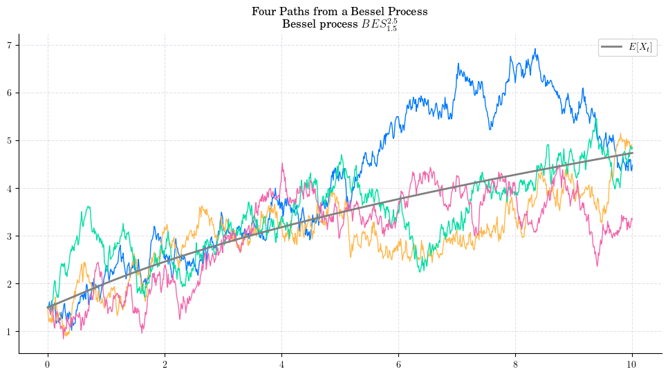
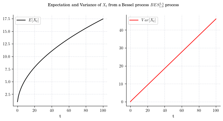
8.3.1.1. Bessel#
The conditional marginal from a Bessel process \(BES_x^{\delta}\), satisfies
and
That is, both the mean and the variance tend to infinity as \(t\) grows. Besides, these expressions imply that the variance grows faster (at linear rate with respect to \(t\)) than the mean. The next plot illustrates these observations.
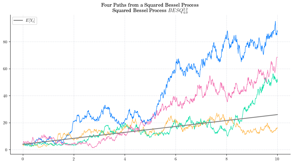
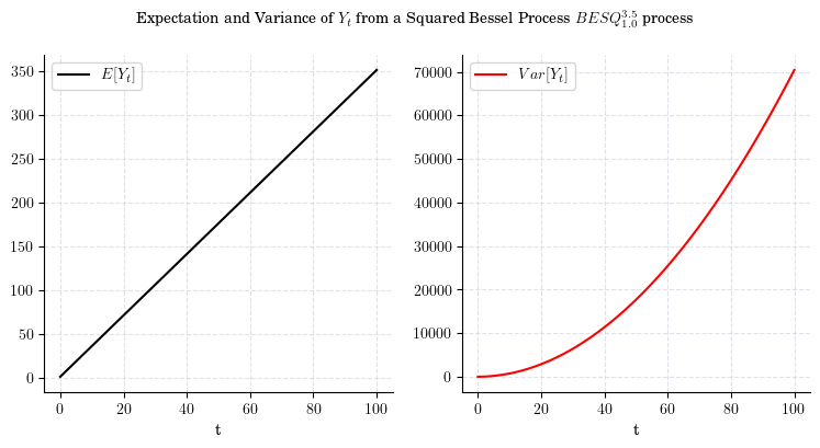
8.3.1.2. Squared Bessel#
The conditional marginal from a Squared Bessel process \(BESQ_0^d\), with integer dimension \(d\geq 2\), satisfies
and
That is, both the mean and the variance tend to infinity as \(t\) grows. Besides, from these equations we can conclude that the variance grows faster than the mean. The next plot illustrates these observations.
8.4. Simulation#
Knowing the distribution of the marginals allows us to simulate paths from Bessel and Squared Bessel processes.
To simulate several paths from Bessel and Squared Bessel processes and visualise them we can use the methods simulate and plot from the aleatory library.
Tip
Remember that the number of points in the partition is defined by the parameter \(n\), while the number of paths is determined by \(N\).
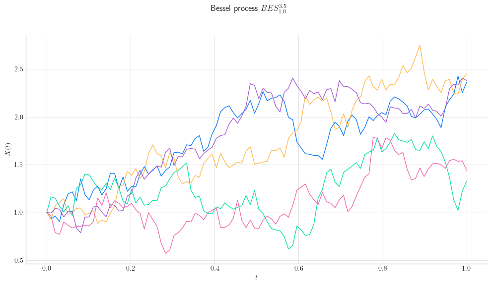
Let’s start by simulating 5 paths from a Bessel Process of dimension 3.5 started at 1.0, over the interval \([0,1]\) using a partition of 100 points. The following snippet shows how to do this by calling the method simulate which returns a list containing the paths as numpy array objects.
# Snippet to Simulate N paths from the Bessel process
from aleatory.processes import BESProcess
bes = BESProcess(dim= 3.5, initial=1.0)
paths = bes.simulate(n=100, N=5)
If we want to simulate and create a simple visualision of the paths, we can use the method plot from the aleatory library.
# Snippet to Simulate and Visualise the paths from the Bessel process
from aleatory.processes import BESProcess
bes = BESProcess(dim= 3.5, initial=1.0)
fig = bes.plot(n=100, N=5)
Similarly, let’s simulate 5 paths from a Squared Bessel process of dimension 6.5 and initial point 2.0, over the interval \([0,1]\) using a partition of 100 points.
# Snippet to Simulate and Visualise the paths from the Squared Bessel process
from aleatory.processes import BESQProcess
bes = BESQProcess(dim= 6.5, initial=2.0)
fig = bes.plot(n=100, N=5)
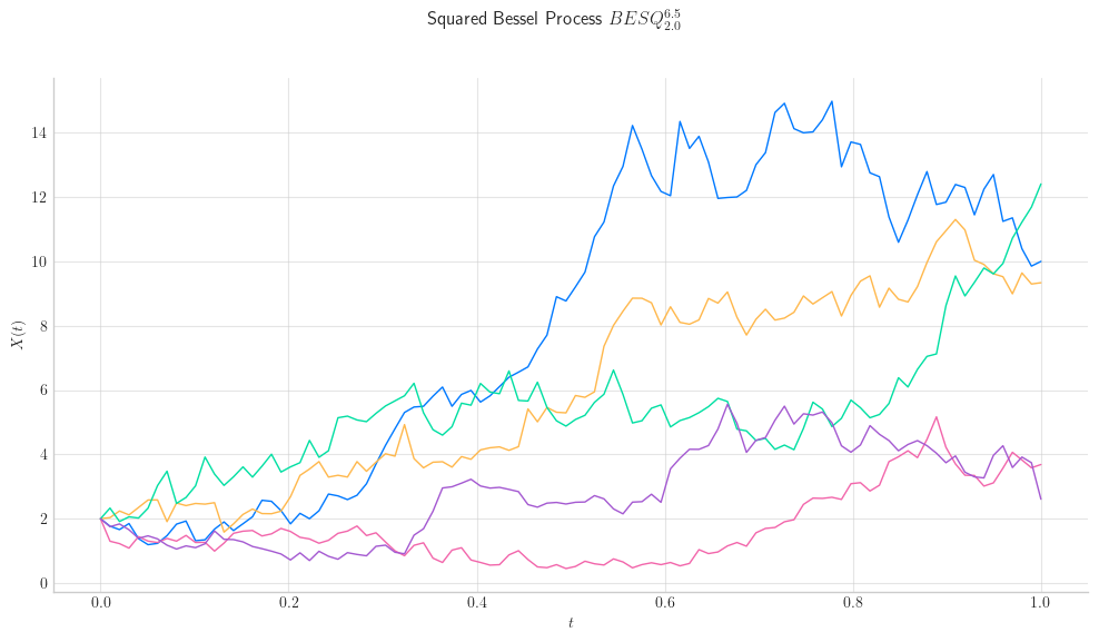
Note
In all plots we are using a linear interpolation to draw the lines between the simulated points.
In the next section, we will see how to create more interesting visualisations!
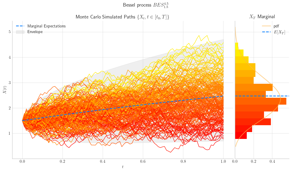
8.5. Final Visualisations#
To finish this note, let us take a look at some simulations.
# from aleatory.processes import BESProcess
bes = BESProcess(dim=4.5, initial=1.5, T=1)
fig = bes.draw(n=100, N=200, envelope=True, colormap="autumn", figsize=(12,6))
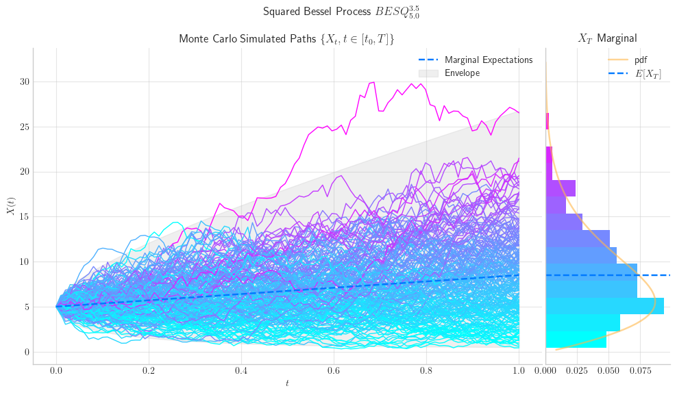
# from aleatory.processes import BESQProcess
bes = BESQProcess(dim=3.5, initial=5.0, T=1.0)
fig = bes.draw(n=100, N=200, envelope=True, colormap="cool")