4. Vasicek Model/Process

The purpose of this notebook is to provide an illustration of the Vasicek Model/Processs and some of its main properties.

Before diving into the theory, let’s start by loading the libraries

• matplotlib

• aleatory

together with the style sheet Quant-Pastel Light.

These tools will help us to make insightful visualisations.

import matplotlib.pyplot as plt
mystyle = "https://raw.githubusercontent.com/quantgirluk/matplotlib-stylesheets/main/quant-pastel-light.mplstyle"
plt.style.use(mystyle)
plt.rcParams["figure.figsize"] = (12, 6)

from aleatory.processes import Vasicek
process = Vasicek(theta=0.5, mu=-10.0, sigma=2.0, initial=1.0, T=20.0)
process.draw(n=200, N=200, envelope=False, title='Vasicek Process')
plt.show()

4.1. Definition

The Vasicek model specifies that the instantaneous interest rate is defined by a stochastic process which can be defined by the following Stochastic Differential Equation (SDE)

(4.1)\[\begin{equation} dX_t = \theta (\mu - X_t) dt + \sigma dW_t, \quad t >0, \end{equation}\]

with initial condition \(X_0 =x_0\in\mathbb{R}\), and where \(W_t\) is a standard Brownian motion, and the three parameters are constants:

• \(\theta>0\) : speed or mean reversion coefficient

• \(\mu \in \mathbb{R}\) : long term mean

• \(\sigma>0\) : volatility

In order to find the solution to this SDE, let us set the function \(f(t,x) = x e^{\theta t}\). Then, Ito’s formula implies

\[\begin{align*} X_te^{\theta t} &= x_0 +\int_0^t X_s \theta e^{\theta s}ds + \int_0^t e^{\theta s}dX_s \\ & = x_0 + \int_0^t \left[ \theta X_s e^{\theta s} +\theta e^{\theta s}(\mu - X_s)\right] ds + \int_0^t e^{\theta s}\sigma dW_s\\ & = x_0 + \int_0^t \left[ \theta e^{\theta s}\mu\right] ds + \int_0^t e^{\theta s}\sigma dW_s\\ & = x_0 + \mu(e^{\theta t} - 1) + \int_0^t e^{\theta s}\sigma dW_s. \end{align*}\]

Thus

(4.2)\[\begin{equation} X_t = x_0e^{-\theta t} + \mu(1- e^{-\theta t}) + \sigma \int_0^t e^{-\theta (t-s)}dW_s. \end{equation}\]

Note

📝 The last expression implies that the process can take positive and negative values.

4.2. Marginal Distributions

Equation (4.2) implies that for each \(t>0\), the variable \(X_t\) follows a normal distribution –since it can be expressed as the sum of a deterministic part and the integral of a deterministic function with respect to the Brownian motion.

Moreover, using the properties of the Brownian Motion we can obtain the following expressions for its expectation and variance.

4.2.1. Expectation and Variance

For each \(t>0\), the conditional marginal \(X_t|X_0\) from a Vacisek process satisfies

\[\begin{equation*} \mathbf{E} [X_t ] = \mathbb{E}[X_t|X_0] = x_0e^{-\theta t} + \mu(1- e^{-\theta t}), \end{equation*}\]

and

\[\begin{equation*} \mathbf{Var} [X_t ] = \mathbb{Var} [X_t |X_0] = \frac{\sigma^2}{ 2\theta} (1- e^{-2\theta t}). \end{equation*}\]

To obtain the expectation we simply use the linearity of the expectation and the fact that the Ito integral in equation (2) is a martingale. Similarly, for the variance we use basic properties of the variance and the isometry property of the Ito integral.

Hence, for each \(t>0\), we have

\[\begin{equation*} X_t \sim \mathcal{N}\left(x_0e^{-\theta t} + \mu(1- e^{-\theta t}), \frac{\sigma}{ \sqrt{2\theta}} \sqrt{ (1- e^{-2\theta t})} \right). \end{equation*}\]

4.2.2. Covariance

In addition, we can verify that

\[Cov(X_t, X_s ) = \frac{\sigma^2 }{ 2\theta}e^{-\theta (t+s)} (e^{2\theta \min\{t,s\}}-1),\]

for any give \(t,s >0.\)

4.2.3. Python Implementation

So, for given \(x_0, \theta>0, \mu, \sigma>0\) and \(t,s>0\) we can implement the above formulas for the expectation, variance, and covariance as follows.

import numpy as np

x0 = 2.0
theta = 1.0
mu = 3.0
sigma = 0.5
t= 10
s = 5

exp = x0*np.exp(-1.0*theta*t) +  mu*(1.0 - np.exp(-1.0*theta*t))
var = sigma**2/(2.0*theta)*(1 - np.exp(-2.0*theta*t)) 
cov = sigma**2/(2.0*theta)*np.exp(-1.0*(t+s))*(np.exp(2.0*theta*(np.min([t,s]))) - 1.0) 

print(f'For x_0={x0}' , f'theta={theta}',f'mu={mu}', f'sigma=.{sigma}', f't={t}', f's={s}', sep=", ")
print(f'E[X_t]= {exp: .6f}')
print(f'Var[X_t]={var :.2f}')
print(f'Cov[X_t, X_s]={cov :.6f}')

For x_0=2.0, theta=1.0, mu=3.0, sigma=.0.5, t=10, s=5
E[X_t]=  2.999955
Var[X_t]=0.12
Cov[X_t, X_s]=0.000842

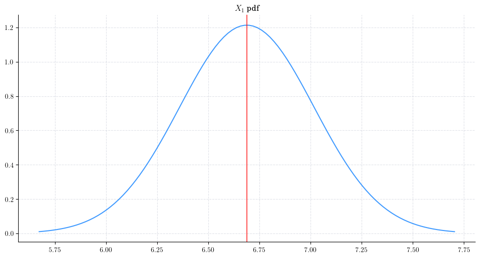
4.2.4. Marginal Distributions in Python

Knowing the distribution –with its corresponding parameters– of the marginal distributions allows us to reproduce them with Python.

One way to do this is by using the object norm from the library scipy.stats. The next cell shows how to create \(X_1\) using this method.

from scipy.stats import norm
import numpy as np 


x0 = 2.0 
theta = 1.0
mu = 3.0
sigma = 0.5
t =1.0 

X_1 = norm(loc=(x0*np.exp(-1.0*theta*t)  + mu*(1.0 - np.exp(-1.0*theta*t))), 
           scale= np.sqrt( (sigma**2/(2.0*theta)*(1 - np.exp(-2.0*theta*t)) )) )

# Now we can calculate the mean and the variance of X_1
print(X_1.mean()) 
print(X_1.var())

2.6321205588285577
0.1080830895954234

Another way to do this is by creating an object Vasicek from aleatory.processes and calling the method get_marginal on it. The next cell shows how to create the marginal \(X_1\) using this method.

from aleatory.processes import Vasicek

x0 = 2.0 
theta = 1.0
mu = 3.0
sigma = 0.5
t =1.0 

process = Vasicek(theta=theta, mu=mu, sigma=sigma, initial=x0)
X_1 = process.get_marginal(t=1)

# Now we can calculate the mean and the variance of X_1
print(X_1.mean())
print(X_1.var())

2.6321205588285577
0.1080830895954234

Hereafter, we will use the latter method to create marginal distributions from the Vacisek process.

4.2.5. Probability Density Functions

The probability density function (pdf) of the marginal distribution \(X_t\) is given by the following expression

\[\begin{equation*} f(x, t; \theta, \mu, \sigma, x_0) = \dfrac{1}{ \frac{\sigma}{ \sqrt{2\theta}} \sqrt{ (1- e^{-2\theta t})} \sqrt{2 \pi }}\exp\left\{ -\dfrac{1}{2} \left(\dfrac{x- [x_0e^{-\theta t} + \mu(1- e^{-\theta t})] }{ \frac{\sigma}{ \sqrt{2\theta}} \sqrt{ (1- e^{-2\theta t})}}\right)^2 \right\}, \qquad \forall x\in\mathbb{R}, t>0. \end{equation*}\]

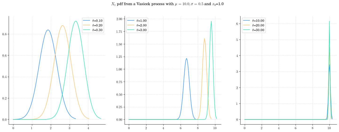
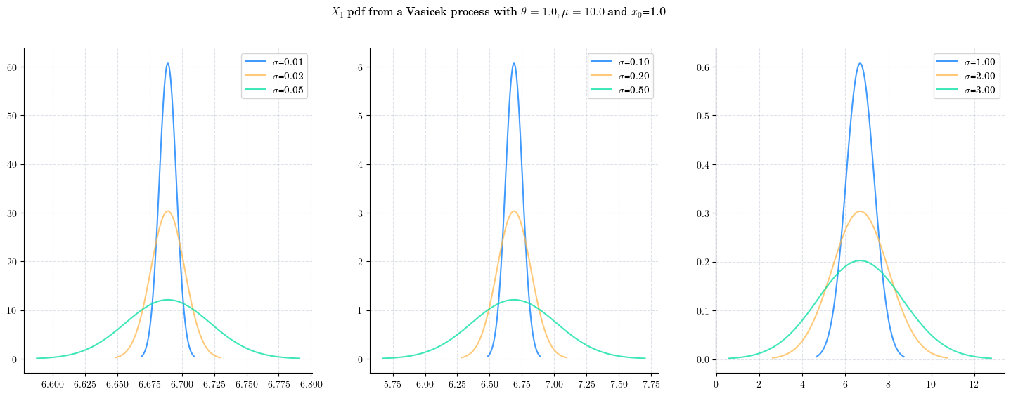
Let’s take a look at the density function of \(X_1\) for different values of \(\theta\), \(\mu\), and \(\sigma\).

First we consider the process Vasicek(theta=1.0, mu=10.0, sigma=0.5, initial=1.0) and plot the marginal density of \(X_1\). Note that the mean is still far from the long term mean \(\mu=10\).

process = Vasicek(theta=1.0, mu=10.0, sigma=0.5, initial=1.0)
X_1 = process.get_marginal(t=1)
x = np.linspace(X_1.ppf(0.001), X_1.ppf(0.999), 100)
plt.plot(x, X_1.pdf(x), '-', lw=1.5, alpha=0.75, label=f'$t$={1:.2f}')
plt.axvline(x = X_1.mean(), color='red', label='$E[X_1]$')
plt.title(f'$X_1$ pdf')
plt.show()

Next we vary the value of the parameter \(\theta\) (the speed of reversion) Vasicek(theta=theta, mu=10.0, sigma=0.5, initial=1.0) and again plot the densities of \(X_1\). Note how the value of \(\theta\) impacts both the mean and the variance of the density.

As \(\theta\) increases:

• The expectation goes from being close to the initial point \(x_0 = 1.0\) to being close to the long term mean \(\mu=10.0\).

• The variance decreases and the distribution becomes more concentrated around the mean.

fig, axs = plt.subplots(1, 3, figsize=(18, 6))
theta_values = ( [0.1, 0.2, 0.3], [1, 2, 3], [10, 20, 30])
for (thetas, ax) in zip(theta_values, axs):
    for theta in thetas:
        process = Vasicek(theta=theta, mu=10.0, sigma=0.5, initial=1.0)
        X_t = process.get_marginal(t=1.0)
        x = np.linspace(0, X_t.ppf(0.999), 100)
        ax.plot(x, X_t.pdf(x), '-', lw=1.5,
                alpha=0.75, label=f'$\\theta$={theta:.2f}')
        ax.legend()
fig.suptitle(r'$X_1$ pdf from a Vasicek process with $\mu = 10.0, \sigma=0.5$ and $x_0$=1.0')
plt.show()

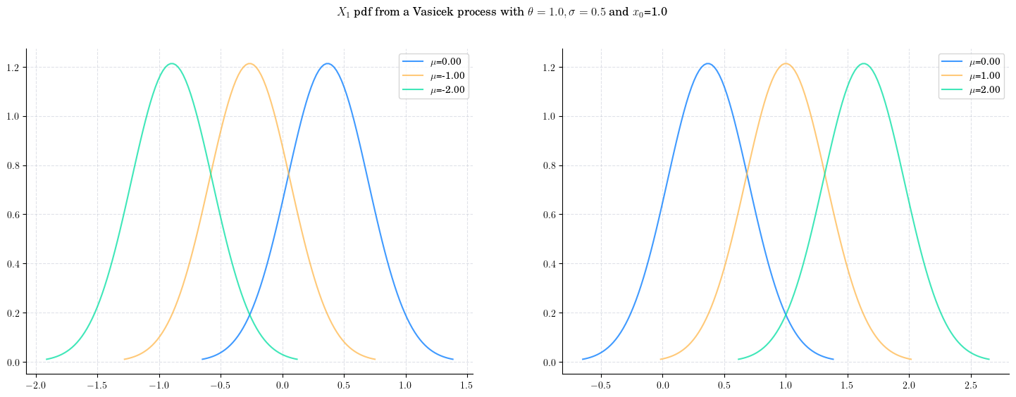
Next we vary the value of the parameter \(\mu\) (the long term mean) in Vasicek(theta=1.0, mu=mu, sigma=0.5, initial=1.0) and again plot the densities corresponding to \(X_1\). Note how the value of \(\mu\) impacts only the mean of the density. We can see that the mean of the density follows the direction of the parameter \(\mu\) which is expected since it will converge to it when \(t\) goes to infinity.

fig, axs = plt.subplots(1, 2, figsize=(18, 6))
mu_values = ([ 0, -1, -2,],  [0, 1, 2])
for (mus, ax) in zip(mu_values, axs):
    for mu in mus:
        process = Vasicek(theta=1.0, mu=mu, sigma=0.5, initial=1.0)
        X_t = process.get_marginal(t=1.0)
        x = np.linspace(X_t.ppf(0.001), X_t.ppf(0.999), 100)
        ax.plot(x, X_t.pdf(x), '-', lw=1.5,
                alpha=0.75, label=f'$\mu$={mu:.2f}')
        ax.legend()
fig.suptitle(r'$X_1$ pdf from a Vasicek process with $\theta = 1.0, \sigma=0.5$ and $x_0$=1.0')
plt.show()

Next we vary the value of the parameter \(\sigma\) (the volatility) in Vasicek(theta=1.0, mu=10.0, sigma=sigma, initial=1.0) and again plot the densities of \(X_1\). Note that the value of \(\sigma\) impacts only the variance of the density while the mean remains constant. As \(\sigma\) increases the variance of \(X_1\) increases and the distribution becomes wider. We can see this by looking at the range in the x-axis of the plots.

fig, axs = plt.subplots(1, 3, figsize=(18, 6))
sigma_values = ([0.01, 0.02, 0.05], [0.1, 0.2,  0.5], [1, 2, 3])
for (sigmas, ax) in zip(sigma_values, axs):
    for sigma in sigmas:
        process = Vasicek(theta=1.0, mu=10.0, sigma=sigma, initial=1.0)
        X_t = process.get_marginal(t=1.0)
        x = np.linspace(X_t.ppf(0.001), X_t.ppf(0.999), 100)
        ax.plot(x, X_t.pdf(x), '-', lw=1.5,
                alpha=0.75, label=f'$\sigma$={sigma:.2f}')
        ax.legend()
fig.suptitle(r'$X_1$ pdf from a Vasicek process with $\theta = 1.0, \mu=10.0$ and $x_0$=1.0')
plt.show()

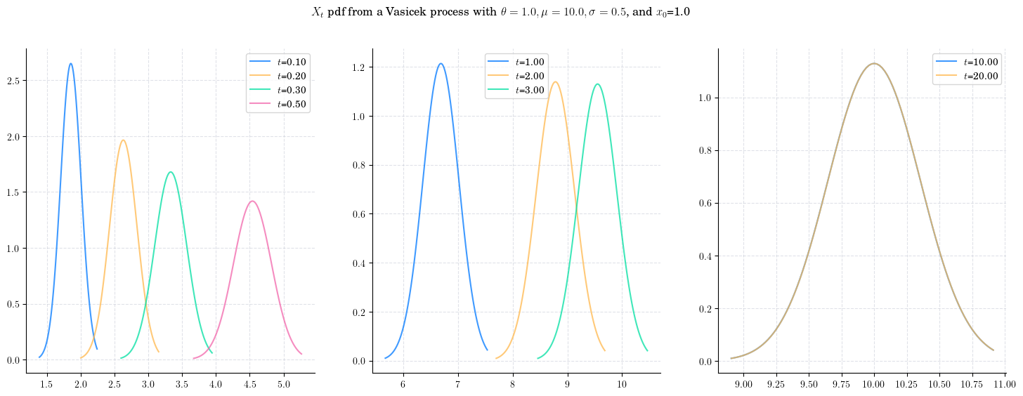
Finally, we will keep all parameters fixed in Vasicek(theta=1.0, mu=10.0, sigma=0.5, initial=1.0) and now plot the densities of \(X_t\) for several values of \(t\). Note how varying \(t\) would impact both the mean and the variance of the density.

As \(t\) increases:

• The expectation goes from being close to the initial point \(x_0 = 1.0\) to being close to the long term mean \(\mu=10.0\).

• The variance also increases but note that it seems to stabilise. We can see this especially in the third graph.

process = Vasicek(theta=1.0, mu=10.0, sigma=0.5, initial=1.0)
fig, axs = plt.subplots(1, 3, figsize=(18, 6))
t_values = ([0.1, 0.2,  0.3, 0.5], [1, 2, 3], [10, 20])
for (ts, ax) in zip(t_values, axs):
    for t in ts:
        X_t = process.get_marginal(t=t)
        x = np.linspace(X_t.ppf(0.001), X_t.ppf(0.995), 100)
        ax.plot(x, X_t.pdf(x), '-', lw=1.5,
                alpha=0.75, label=f'$t$={t:.2f}')
        ax.legend()
fig.suptitle(r'$X_t$ pdf from a Vasicek process with $\theta = 1.0, \mu=10.0, \sigma=0.5$, and $x_0$=1.0')
plt.show()

4.2.6. Sampling

Now, let’s see how to get a random sample from \(X_t\) for any \(t>0\).

The next cell shows how to get a sample of size 5 from \(X_1\).

# from aleatory.processes import Vasicek
process = Vasicek(theta=1.0, mu=10.0, sigma=0.5, initial=1.0)
X_1= process.get_marginal(t=1.0)
X_1.rvs(size=5)

array([6.92652129, 6.39524409, 6.73077842, 6.65327447, 7.12773049])

Similarly, we can get a sample from \(X_{10}\)

X_10 = process.get_marginal(t=10)
X_10.rvs(size=5)

array([10.06590198,  9.56805405, 10.15120991,  9.44203325, 10.15908188])

4.3. Simulation

In order to simulate paths from a stochastic process, we need to set a discrete partition over an interval for the simulation to take place.

For simplicity, we are going to consider an equidistant partition of size \(n\) over \([0,T]\), i.e.:

\[\begin{equation*} t_i = \frac{i}{n-1} T \qquad \hbox{for } i = 0, \cdots, n-1. \end{equation*}\]

Then, the goal is to simulate a path of the form \(\{ X_{t_i} , i=0,\cdots, n-1\}\). We will use Euler-Maruyama approximation.

4.3.1. Simulating and Visualising Paths

We can simulate several paths from a Vasicek process and visualise them we can use the method plot from the aleatory library.

Let’s simulate 10 paths over the interval \([0,1]\) using a partition of 100 points.

Tip

Remember that the number of points in the partition is defined by the parameter \(n\), while the number of paths is determined by \(N\).

# from aleatory.processes import Vasicek
process = Vasicek(theta=1.0, mu=10.0, sigma=0.5, initial=2.0)
fig = process.plot(n=100, N=10, title='10 paths of the Vasicek Process')

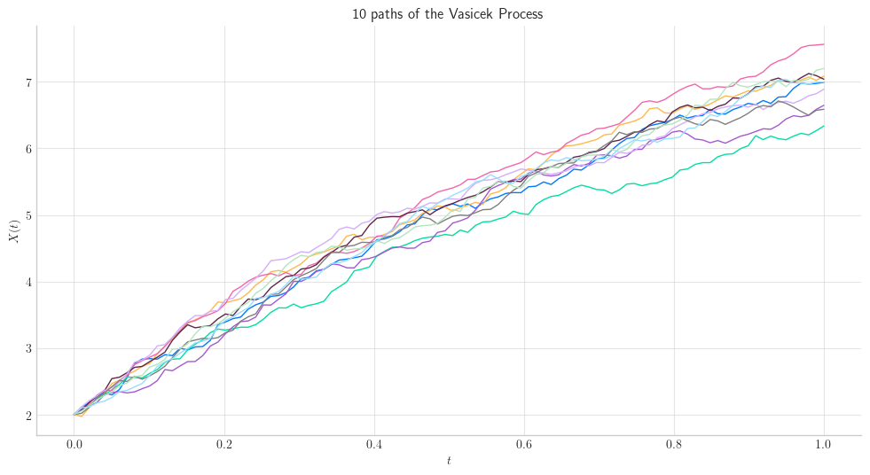
Note

In all plots we are using a linear interpolation to draw the lines between the simulated points.

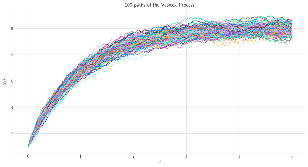
Similarly, we can define the process over the interval \([0, 5]\) and simulate 50 paths with a partition of size 100.

# from aleatory.processes import Vasicek
process = Vasicek(theta=1.0, mu=10.0, sigma=0.5, initial=1.0, T=5.0)
fig = process.plot(n=200, N=100, title='100 paths of the Vasicek Process')

4.4. Long Time Behaviour

4.4.1. Expectation and Variance

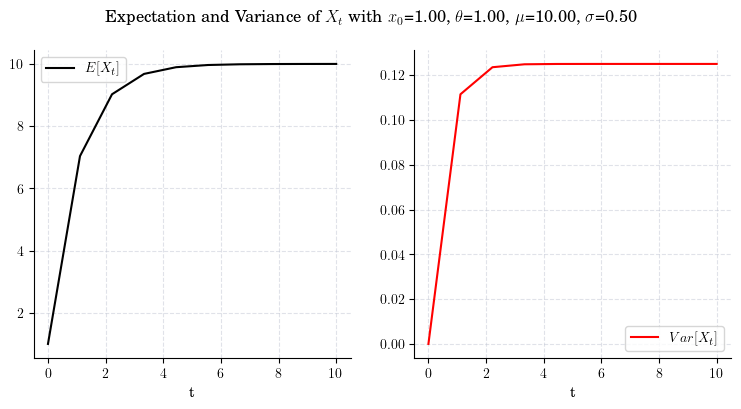
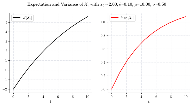
Note that when \(t\) goes to infinity, we have

\[\begin{equation*} \lim_{t\rightarrow\infty} \mathbf{E} [X_t ] = \lim_{t\rightarrow\infty} \left[ x_0e^{-\theta t} + \mu(1- e^{-\theta t}) \right] = \mu. \end{equation*}\]

and

\[\begin{equation*} \lim_{t\rightarrow\infty}\mathbf{Var} [X_t ] = \lim_{t\rightarrow\infty} \frac{\sigma^2}{ 2\theta} (1- e^{-2\theta t}) = \frac{\sigma^2}{ 2\theta}. \end{equation*}\]

Next, we illustrate the convergence of both the mean and the variance of \(X_t\) as \(t\) grows. Note that the speed of convergence is determined by \(\theta\).

def draw_mean_variance(x0, theta, mu, sigma, T=100):

    process = Vasicek(theta=theta, mu=mu, sigma=sigma, initial=x0, T=T)
    ts = np.linspace(0, T, T)
    means = process.marginal_expectation(ts)
    variances = process.marginal_variance(ts)
    fig, (ax1, ax2,) = plt.subplots(1, 2, figsize=(9, 4))
    
    ax1.plot(ts, means, lw=1.5, color='black', label='$E[X_t]$')
    ax1.set_xlabel('t')
    ax1.legend()
    ax2.plot(ts,  variances, lw=1.5, color='red', label='$Var[X_t]$')
    ax2.set_xlabel('t')
    ax2.legend()
    fig.suptitle(
        'Expectation and Variance of $X_t$ with ' f'$x_0$={x0:.2f}, $\\theta$={theta:.2f}, $\mu$={mu:.2f}, $\sigma$={sigma:.2f}', size=12)
    plt.show()

draw_mean_variance(theta=1.0, mu=10.0, sigma=0.5, x0=1.0, T=10)

draw_mean_variance(theta=0.1, mu=10.0, sigma=0.5, x0=-2.0, T=10)

4.4.2. Marginal

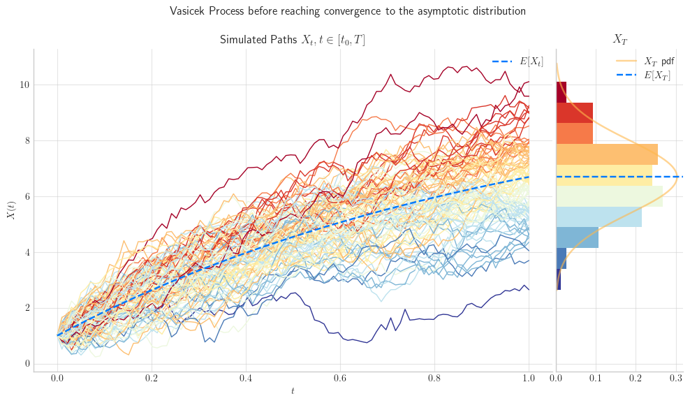
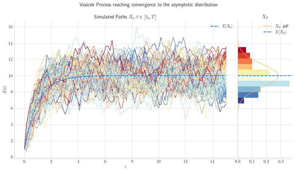
The marginal distribution \(X_t\) given an initial point \(x_0\), converges to

\[\begin{equation*} X_{\infty} \sim \mathcal{N} \left(\mu , \frac{\sigma}{ \sqrt{2\theta} }\right), \end{equation*}\]

as \(t\) goes to infinity. Let’s make some simulations to illustrate this convergence.

First, we simulate 1000 paths from Vasicek(theta=1.0, mu=10.0, sigma=2.0, initial=1.0, T=1.0) over the interval \([0,1]\). Here, we can see the the distribution of \(X_1\) has mean around 6.0. This means that the process has not reached convergence, since we have not arrived to the long term mean \(\mu=10.0\).

# from aleatory.processes import Vasicek
process = Vasicek(theta=1.0, mu=10.0, sigma=2.0, initial=1.0, T=1.0)
fig = process.draw(n=100, N=100, title='Vasicek Process before reaching convergence to the asymptotic distribution')

Now, we simulate 1000 paths from the same process Vasicek(theta=1.0, mu=10.0, sigma=2.0, initial=1.0, T=15) but this time over the interval \([0,15]\). In the picture, we can see the the distribution of \(X_{15}\) has mean equal to the long term mean \(\mu=10\). The process has reached convergence!

# from aleatory.processes import Vasicek
process = Vasicek(theta=1.0, mu=10.0, sigma=2.0, initial=1.0, T=15.0)
fig = process.draw(n=100, N=100, title='Vasicek Process reaching convergence to the asymptotic distribution')

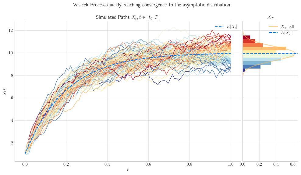
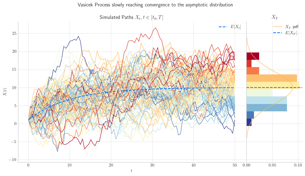
4.4.2.1. The parameter \(\theta\) determines the Speed of Convergence

# from aleatory.processes import Vasicek
process = Vasicek(theta=5.0, mu=10.0, sigma=2.0, initial=1.0, T=1.0)
fig = process.draw(n=100, N=100, title='Vasicek Process quickly reaching convergence to the asymptotic distribution')

process = Vasicek(theta=0.1, mu=10.0, sigma=2.0, initial=1.0, T=50.0)
process.draw(n=100, N=100, title='Vasicek Process slowly reaching convergence to the asymptotic distribution')
plt.show()

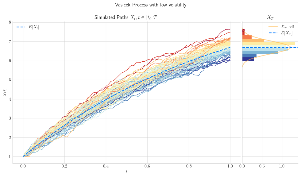
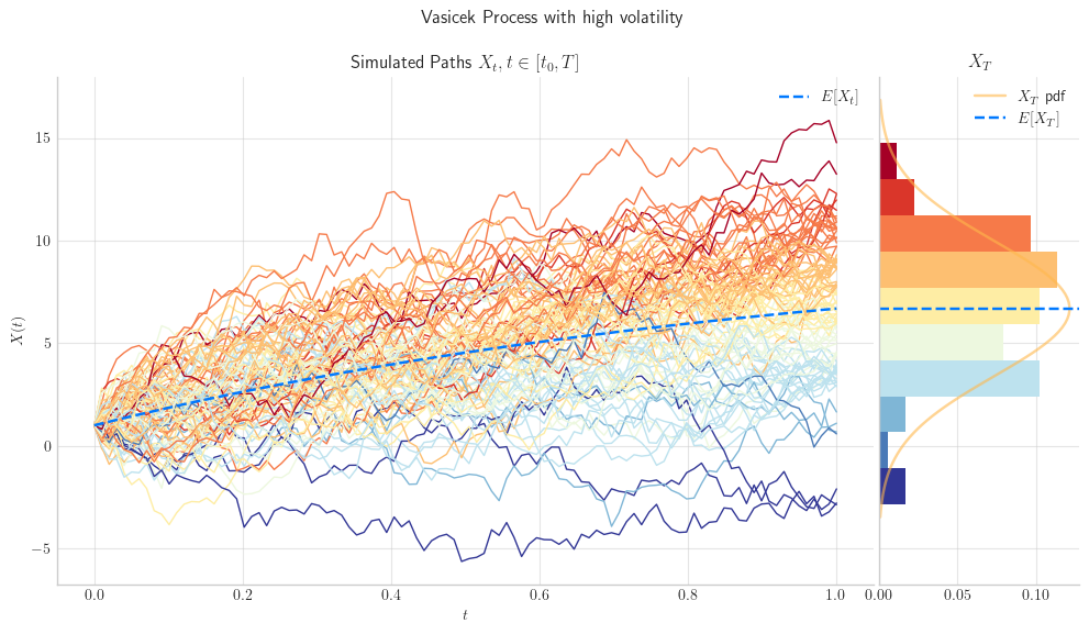
4.4.2.2. The parameter \(\sigma\) determines the volatility in the simulation

# from aleatory.processes import Vasicek
process = Vasicek(theta=1.0, mu=10.0, sigma=0.5, initial=1.0, T=1.0)
fig = process.draw(n=100, N=100, title='Vasicek Process with low volatility')

# from aleatory.processes import Vasicek
process = Vasicek(theta=1.0, mu=10.0, sigma=5.0, initial=1.0, T=1.0)
fig =process.draw(n=100, N=100, title='Vasicek Process with high volatility')

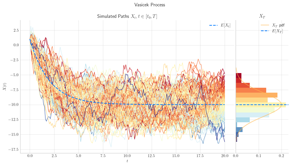
4.5. Visualisation

To finish this note, let’s take a final look at a some simulations from the Vasicek process.

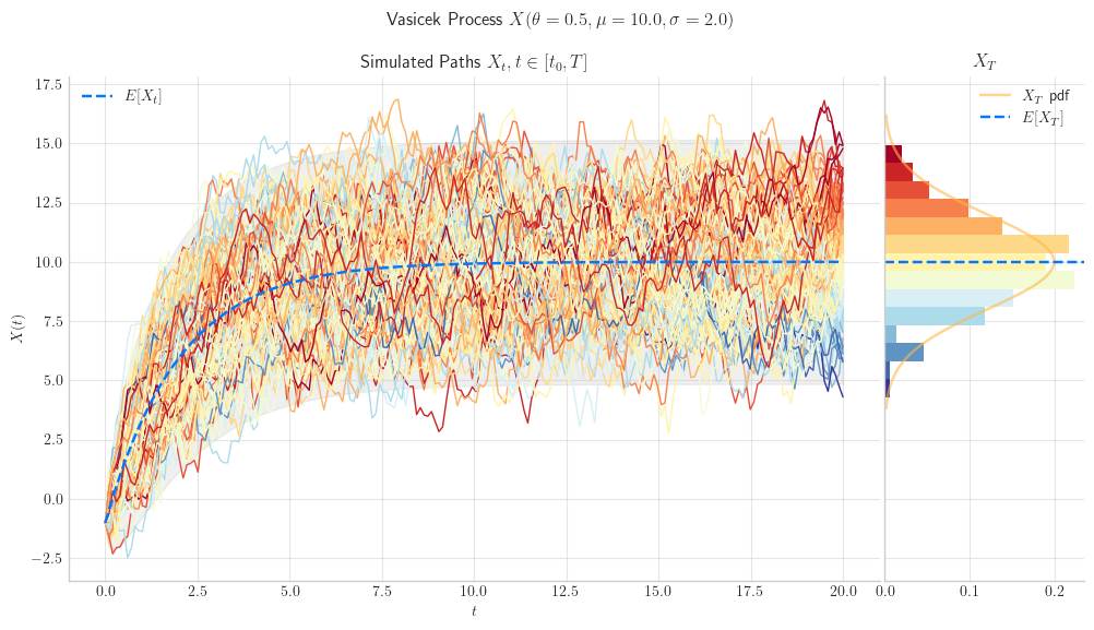
# from aleatory.processes import Vasicek
process = Vasicek(theta=0.5, mu=10.0, sigma=2.0, initial=-1.0, T=20.0)
fig = process.draw(n=200, N=200, envelope=True)

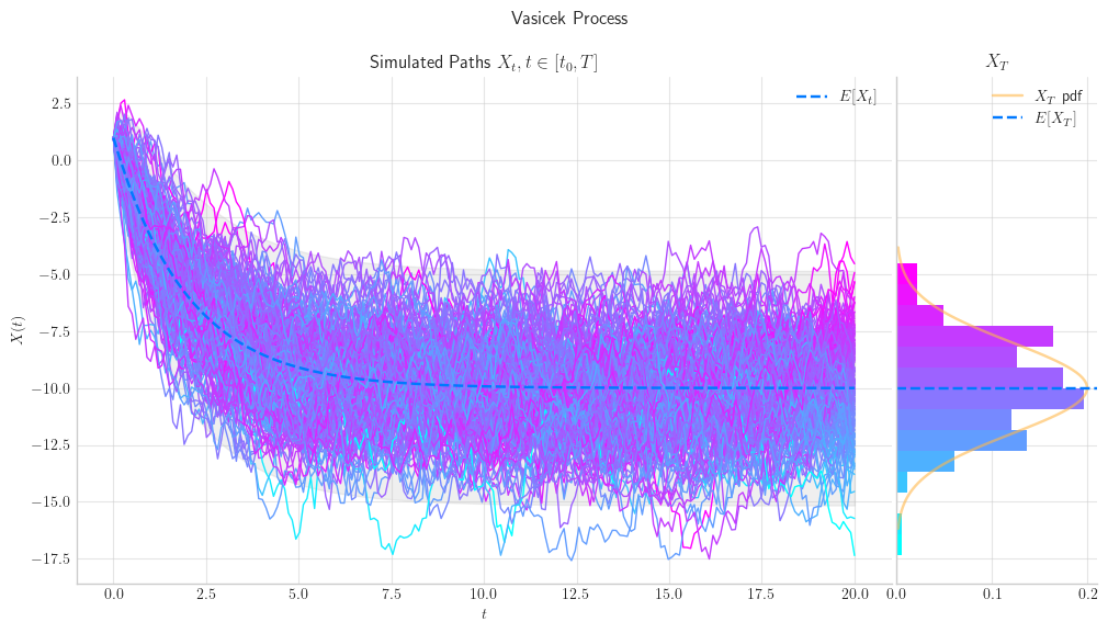
# from aleatory.processes import Vasicek
process = Vasicek(theta=0.5, mu=-10.0, sigma=2.0, initial=1.0, T=20.0)
fig = process.draw(n=200, N=200, envelope=True, colormap="cool", title='Vasicek Process')

# from aleatory.processes import Vasicek
# import matplotlib.pyplot as plt
# import numpy as np

process = Vasicek(theta=1.0, mu=-10.0, sigma=np.sqrt(2), initial=0.0, T=12.0)
path = process.simulate(n=1000, N=1)
ts = process.times
exp = process.marginal_expectation(ts)
plt.plot(ts, path[0], label= f'$x_0$ = 0, $\mu$ = -10')
plt.plot(ts, exp, color='grey',linewidth=2)

for x0 in [-10.0, 0.0, 10.0]:
    process = Vasicek(theta=1.0, mu=0.0, sigma=np.sqrt(2), initial=x0, T=12.0)
    path = process.simulate(n=1000, N=1)
    plt.plot(ts, path[0], label= f'$x_0$ = {x0:.0f}, $\mu$ = 0')
    exp = process.marginal_expectation(ts)
    plt.plot(ts, exp, color='grey', linewidth=2)
plt.plot(ts, exp, color='grey', label=f'$E[X_t]$')
plt.legend()
plt.title('Four Paths from the Vasicek Model\n $dX_t = \\theta(\mu - X_t) dt + \sigma dW_t$\n with $\\theta = 1, \sigma = \sqrt{2}$')
plt.show()

4.6. References and Further Reading

• Damiano Brigo, Fabio Mercurio (2001). Interest Rate Models – Theory and Practice with Smile, Inflation and Credit

• Vasicek, O. (1977). “An equilibrium characterization of the term structure”. Journal of Financial Economics.