
1. Brownian Motion#
The purpose of this notebook is to review and illustrate the standard Brownian motion and some of its main properties.
Before diving into the theory, let’s start by loading the libraries
matplotlib
together with the style sheet Quant-Pastel Light.
These tools will help us to make insightful visualisations.
1.1. Definition#
A standard Brownian motion or Wiener process is a stochastic process \(W =\{W_t, t\geq 0\},\) characterised by the following four properties:
\(W_0 = 0\)
\(W_t-W_s \sim N(0, t-s),\) for any \(0\leq s \leq t\)
\(W\) has independent increments
\(W\) is almost surely continuous.
1.2. Marginal Distributions#
Point (2) in the Brownian motion definition implies that for each \(t>0\), the one dimensional marginal distribution \(W_t\) is normally distributed with expectation zero, and variance equals \(t\), i.e.:
1.2.1. Expectation, Variance, and Covariance#
Equation(1.1) implies that
and
Besides, for any \( t > s >0\), we have
where the second equality follows by simply using the linearity of the expectation and independent increments property. That is
1.2.2. Finite Dimensional Distributions#
Moreover, for any finite set \(t_1 < t_2 < \cdots < t_m\), the vector \((W_{t_1}, W_{t_2}, \cdots, W_{t_m}),\) follows a Mutivariate normal distribution with zero (zero-vector in \(\mathbb{R}^m\)) and covariance matrix
Hereafter, we will focus on the one dimensional marginal distributions \(W_t, t>0\) and will refer to them simply as marginal distributions.
1.2.3. Marginal Distributions in Python#
Knowing the distribution –with its corresponding parameters– of the marginal variables allows us to reproduce them with Python.
One way to do this is by using the object norm from the library scipy.stats.
The next cell shows how to create \(W_1\) using this method.
import numpy as np
from scipy.stats import norm
W_1 = norm(loc=0, scale=np.sqrt(1))
Another way to do this is by creating an object BrownianMotion from aleatory.processes and calling the method get_marginal on it.
The next cell shows how to create the marginal \(W_1\) using this method.
from aleatory.processes import BrownianMotion
process = BrownianMotion()
W_1 = process.get_marginal(t=1)
Hereafter, we will use the latter method to create marginal distributions from Brownian Motion.
1.2.4. Probability Density Functions#
The probability density function (pdf) of the marginal distribution \(W_t\) is given by the following expression
1.2.4.1. Fokker-Planck Equation#
The pdf satisfies the Fokker-Planck equation
1.2.4.2. Visualisation#
In order to visualise these functions, we are going to load the library matplotlib and set some formatting options.
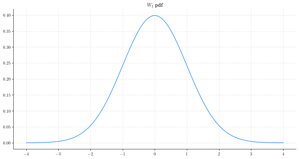
We can plot the pdf of \(W_1\) as follows.
from aleatory.processes import BrownianMotion

process = BrownianMotion()
W_1 = process.get_marginal(t=1)
x = np.linspace(-4, 4,100)
plt.plot(x, W_1.pdf(x), '-', lw=1.5, alpha=0.75, label=f'$t$={1:.2f}')
plt.title(f'$W_1$ pdf')
plt.show()
Next, let’s take a look at the pdfs for different marginal distributions \(W_t\).
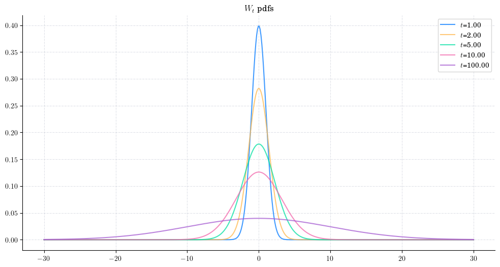
In this chart, we clearly see the characteristic symmetric bell-shaped curves of the normal/Gaussian distribution. Moreover, we can make the following observations:
The Brownian motion will take positive and negative values
The Brownian motion would take bigger (in magnitude) values as \(t\) increases
The marginal distributions of the Brownian Motion flatten/spread as \(t\) increases.
1.2.5. Sampling#
Now, let’s see how to obtain a random sample from the marginal \(W_t\) for \(t>0\).
The next cell shows how to get a sample of size 5 from \(W_1 \sim\mathcal{N}(0,1)\).
from aleatory.processes import BrownianMotion
process = BrownianMotion()
W_t = process.get_marginal(t=1.0)
W_t.rvs(size=5)
array([-1.2381154 , 0.48251085, -0.86619211, -0.00444666, 1.50547328])
Similarly, we can get a sample from \(W_{10} \sim \mathcal{N}(0, \sqrt{10})\), as follows
W_t = process.get_marginal(t=10.0)
W_t.rvs(size=5)
array([ 1.55946711, -1.11685924, -0.70670166, -1.15348188, 2.54626445])
1.3. Simulation#
In order to simulate paths from a stochastic process, we need to set a discrete partition over an interval for the simulation to take place.
For simplicity, we are going to consider an equidistant partition of size \(n\) over \([0,T]\), i.e.:
Then, the goal is to simulate a path of the form \(\{ W_{t_i} , i=0,\cdots, n-1\}\). Of course, there are different ways to do this. Here, we are going to use the fact tha we can express each \(W_{t_i}\) as follows:
Thus, we can built the path by simply simulating from a normal distribution \(\mathcal{N}(0,\frac{T}{n-1})\) and then taking the cumulative sum.
First, we construct the partition, using np.linspace, and calculate the standard deviation of the normal random variable \(\mathcal{N}(0, \frac{T}{n-1})\), i.e.:
import numpy as np

T = 1.0 # End point of the interval to simulate [O,T]
n = 100 # Number of points in the partition
times = np.linspace(0, T, n) # Partition
sigma = np.sqrt( T/(n-1) ) # Standard Deviation
print(sigma)
0.10050378152592121
Next, we generate a sample of size \(n-1\) from the random variable \(\mathcal{N}(0, \frac{T}{n-1})\), and calculate the cumulative sum.
from scipy.stats import norm

normal_increments = norm.rvs(loc=0, scale=sigma, size=n-1) # Sample of size n-1
normal_increments = np.insert(normal_increments, 0, 0) # This is the initial point
Wt = normal_increments.cumsum() # Taking the cumulative sum
Note
Note that we had to add the initial point of the Brownian motion.
Putting these steps together we get the following snippet
# Snippet to Simulate Brownian Motion
import numpy as np
from scipy.stats import norm

T = 1.0 # End point of the interval to simulate [O,T]
n = 100 # Number of points in the partition
times = np.linspace(0, T, n) # Partition
sigma = np.sqrt( T/(n-1) ) # Standard Deviation

normal_increments = norm.rvs(loc=0, scale=sigma, size=n-1) # Sample of size n-1
normal_increments = np.insert(normal_increments, 0, 0) # Adding the initial point
Wt = normal_increments.cumsum() # Taking the cumulative sum
Let’s plot our simulated path!
plt.plot(times, Wt, 'o-', lw=1)
plt.title('Brownian Motion Path')
plt.show()
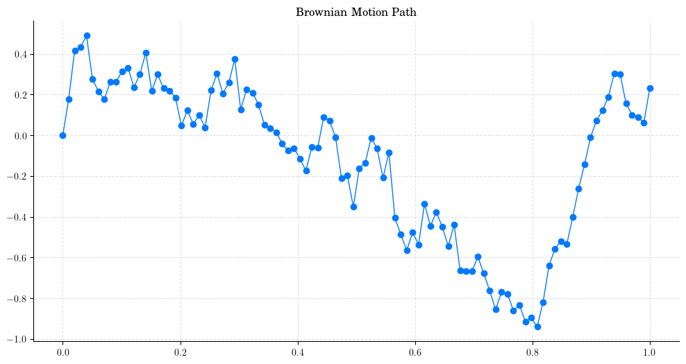
Note
In this plot, we are using a linear interpolation to draw the lines between the simulated points.
1.3.1. Simulate and Visualise Paths#
To simulate several paths from a Brownian Motion and visualise them we can use the method plot from the aleatory library.
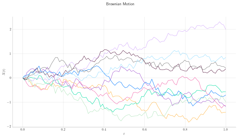
Let’s simulate 10 paths over the interval \([0,1]\) using a partition of 100 points.
Tip
Remember that the number of points in the partition is defined by the parameter \(n\), while the number of paths is determined by \(N\).
from aleatory.processes import BrownianMotion

process = BrownianMotion()
process.plot(n=100, N=10)
plt.show()
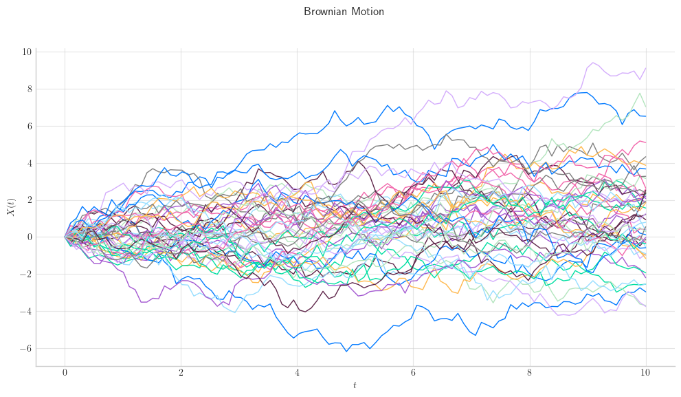
Similarly, we can define the Brownian Motion over the interval \([0, 10]\) and simulate 50 paths with a partition of size 100.
process = BrownianMotion(T=10)
process.plot(n=100, N=50)
plt.show()
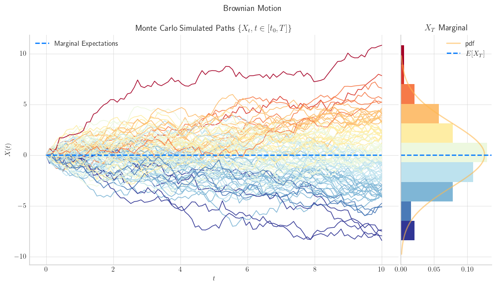
process.draw(n=100, N=100)
plt.show()
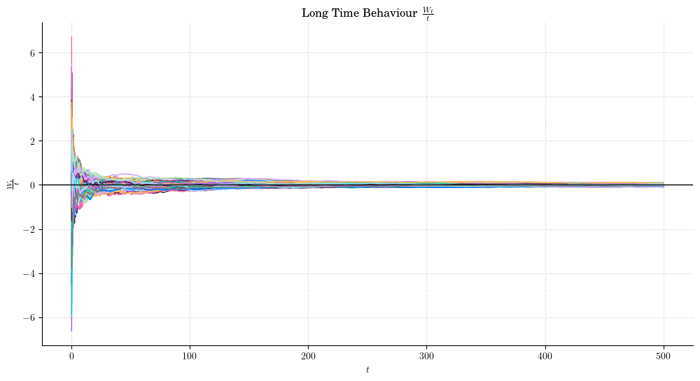
1.4. Long Time Behaviour#
Almost surely
This property is the analogous of the Law of Large Numbers and sometimes is referred as such.
We can visualise this phenomenon by simulating trajectories of the Brownian Motion over a long interval and then simply plottling the values \(\frac{W_t}{t}\). Let’s try to do this over the interval \([0, 500]\)
process = BrownianMotion(T=500)
paths = process.simulate(n=5000, N=100)
t = process.times
We can zoom-in to see the what was happening when \(t\) was not that big e.g. over the interval \([0,5]\)
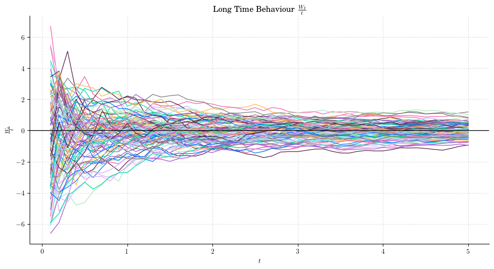
We can see that the ratio \(\frac{W_t}{t}\) is definitely going towards zero but not quite there yet at \(t=5\).
Now, let’s zoom in on the last part of the interval \([0, 500]\), e.g. on \([400, 500]\)
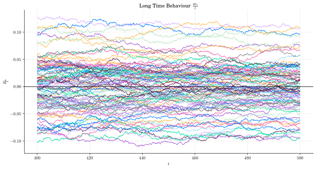
Here we can see that the ratio is much closer to zero (around \(\pm 0.1\)) than before! Of course, we are still not quite there yet, but convergence is definitely happening.
1.5. Reflection Principle#
For any point \(a>0\), we have
This states that if the path of a Brownian Motion reaches a value \(a>0\) at some time \(s\), then the subsequent path has the same distribution as its reflection about the level of \(a\).
The following picture illustrates this behaviour with \(a=1\). The reflected path \(W^{\ast}\) is shown in yellow. Refection principle states that after the crossing point, both paths have the same distribution.
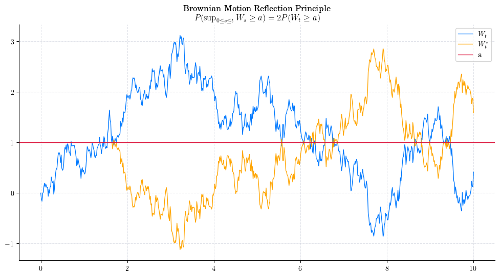
You can find the proof here: Reflection Principle (Wiener process)- Wiki.
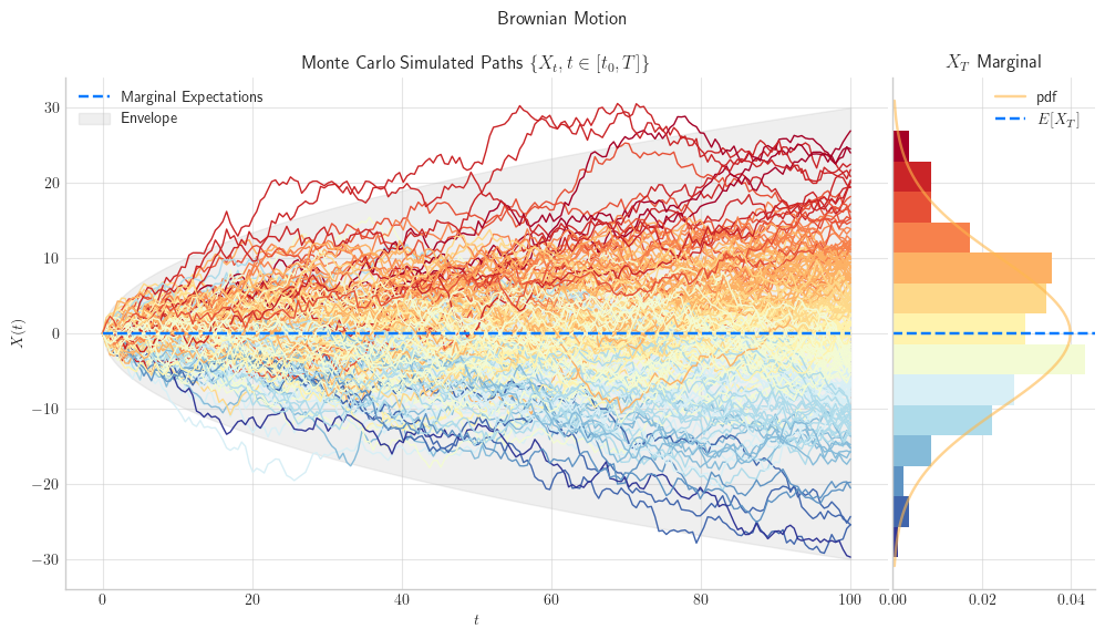
1.6. Visualisation#
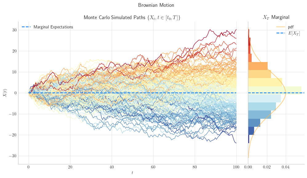
To finish this note, let’s take a final look at a simulation from the Brownian Motion.
# Snippte to simulate N paths from a Brownian Motion defined over [0,1] (each path with n steps)
from aleatory.processes import BrownianMotion
process = BrownianMotion(T=100)
process.draw(n=200, N=200, envelope=True)
plt.show()
1.7. References and Further Reading#
The Brownian Movement by Feynman, R. (1964) in “The Feynman Lectures of Physics”, Volume I. pp. 41–1.
Brownian Motion and Stochastic Calculus by Ioannis Karatzas, and Steven E. Shreve (1998), Springer.
Brownian Motion Notes by Peter Morters and Yuval Peres (2008).
The Zero Set and Arcsine Laws of Brownian Motion by Lecturer: Manjunath Krishnapur.