Day 12 : Ornstein-Uhlenbeck#
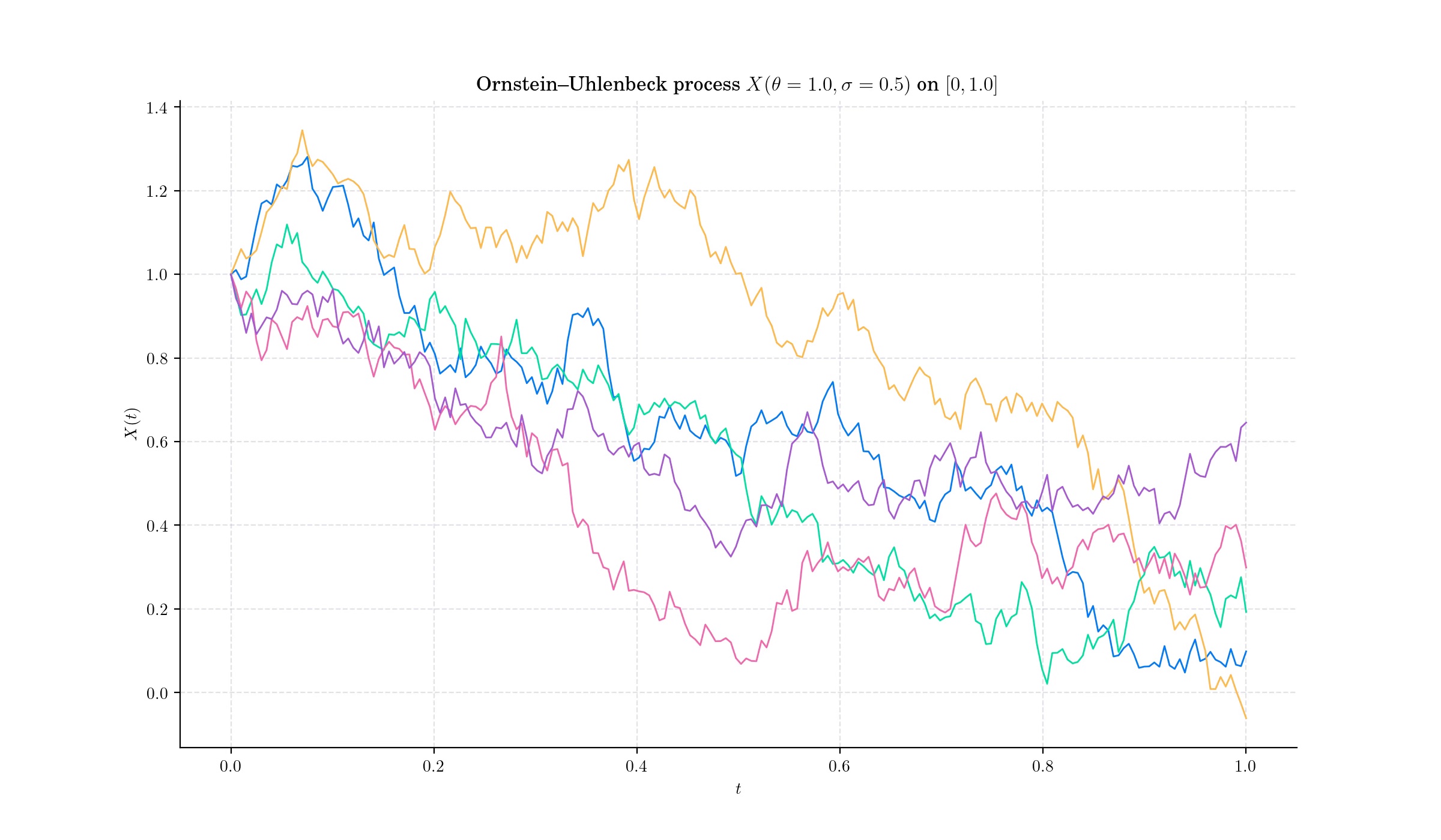
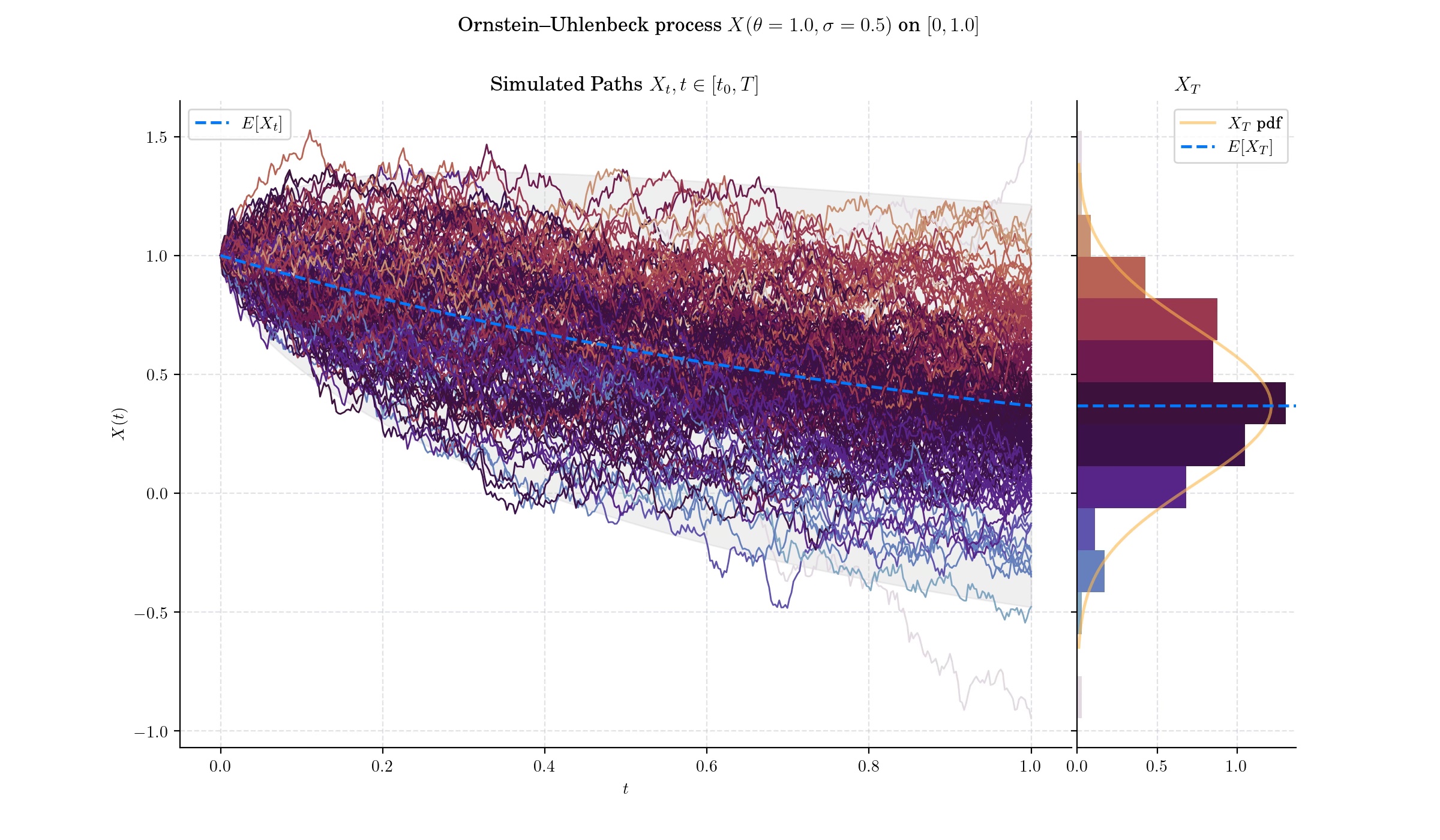
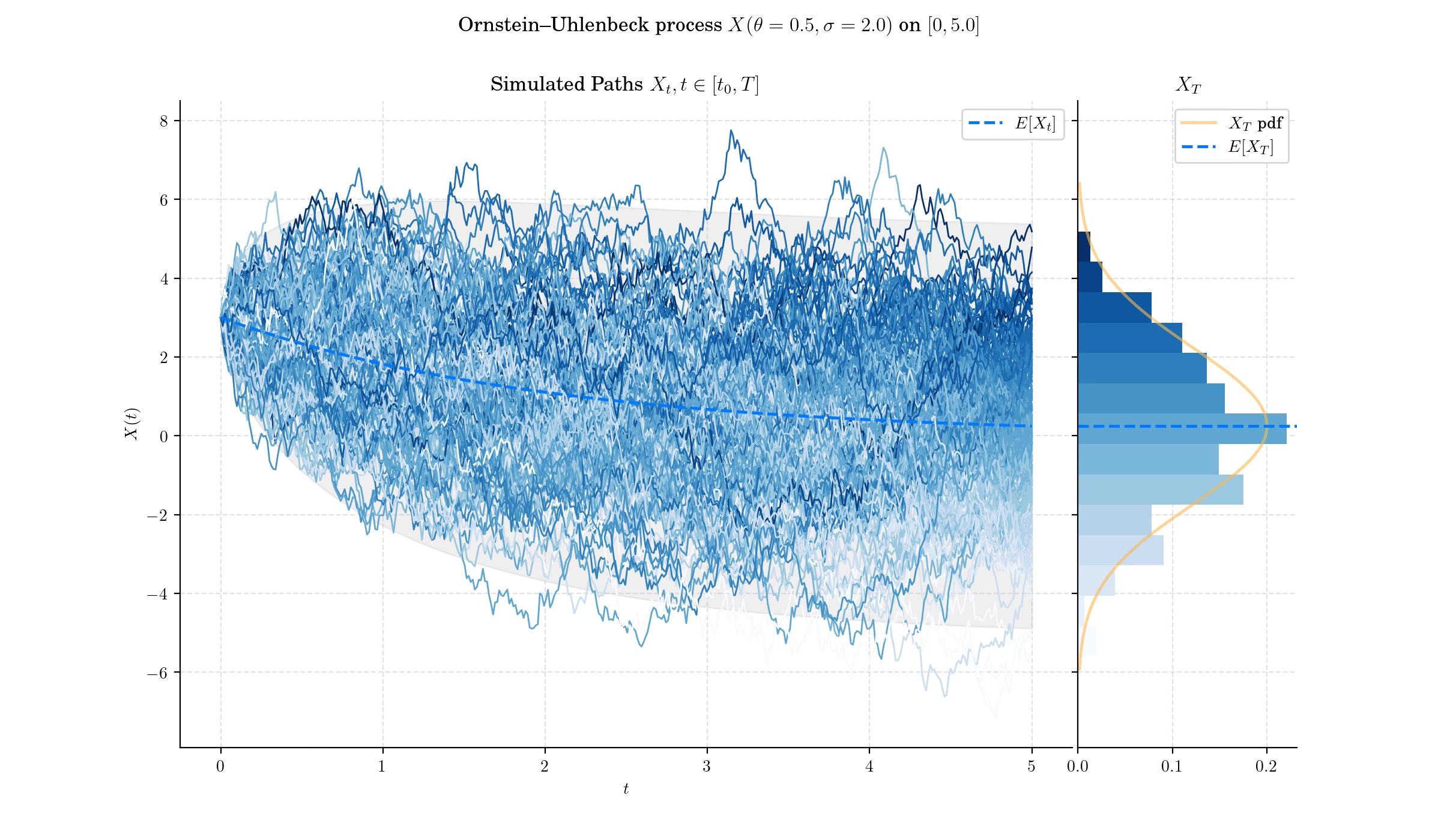
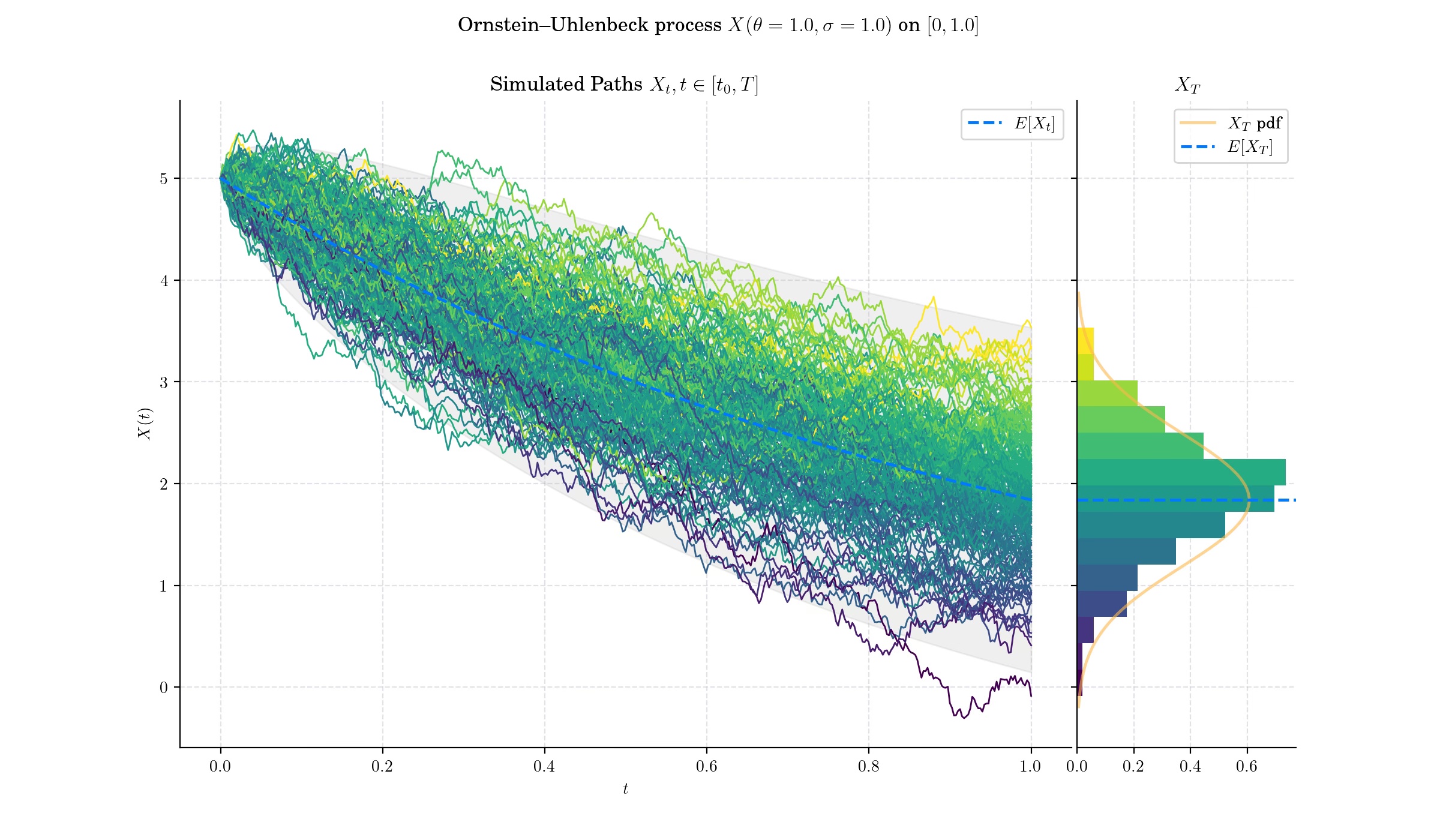
The Ornstein-Uhlenbeck (OU) process is a stochastic process that plays a critical role in fields like physics, finance, and biology. It is a type of Gaussian process known for its mean-reverting properties, making it particularly useful for modelling phenomena that oscillate around a long-term average.
Definition#
The Ornstein–Uhlenbeck process \(X=\{X(t) : t\geq 0\}\) is defined by the following stochastic differential equation:
with initial condition \(X(0) = x\_0\); where \(\theta>0\) and \(\sigma >0\) are constant parameters and \(W\) denotes the Wiener process. In order to find the solution to this SDE, let us set the function \(f(t,x) = x e^{\theta t}\). Then, Ito’s formula implies
Thus
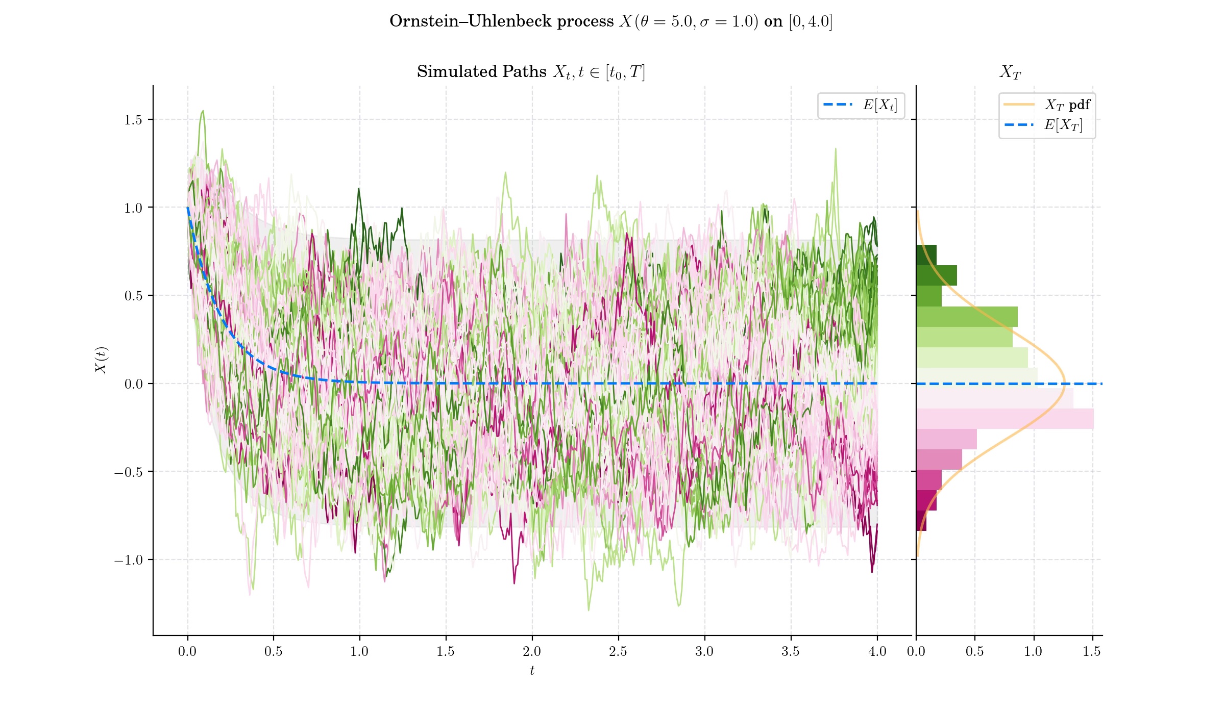
This expression implies that for each \(t>0\), the random variable \(X\_t\) follows a normal distribution –since it can be expressed as the sum of a deterministic part and the integral of a deterministic function with respect to the Brownian motion.
🔔 Random Facts 🔔#
The process was introduced by physicists Leonard Ornstein and George Eugene Uhlenbeck in 1930 to describe the velocity of a massive particle undergoing Brownian motion in a viscous fluid.
The Ornstein–Uhlenbeck process is a stationary Gauss–Markov process, which means that it is a Gaussian process, a Markov process, and is temporally homogeneous. In fact, it is the only nontrivial process that satisfies these three conditions, up to allowing linear transformations of the space and time variables.
The Ornstein–Uhlenbeck process can also be considered as the continuous-time analogue of the discrete-time AR(1) process.
The Ornstein–Uhlenbeck process can also be described in terms of a probability density function, \(f(x,t),\) which specifies the probability of finding the process in the state \(x\) at time \(t\). This function satisfies the Fokker–Planck equation
The Ornstein–Uhlenbeck process (and its variations) is widely used to model interest rates, currency exchange rates, and commodity prices.
More to Read 📚#
Doob, J. L. “The Brownian Movement and Stochastic Equations.” Annals of Mathematics, vol. 43, no. 2, 1942, pp. 351–69. JSTOR, https://doi.org/10.2307/1968873. Accessed 12 Dec. 2024.
Jacobsen, Martin. “Laplace and the Origin of the Ornstein-Uhlenbeck Process.” Bernoulli, vol. 2, no. 3, 1996, pp. 271–86. JSTOR, https://doi.org/10.2307/3318524. Accessed 12 Dec. 2024.
Risken, H. (1989). The Fokker–Planck Equation: Methods of Solution and Applications. New York: Springer-Verlag. ISBN 978-0387504988.
Patrick Cheridito. Hideyuki Kawaguchi. Makoto Maejima. “Fractional Ornstein-Uhlenbeck processes.”Electron. J. Probab. 8 1 - 14, 2003. https://doi.org/10.1214/EJP.v8-125
P.s. If you are curious about probability distributions visit the Advent Calendar 2023 ✨