Day 5: Arithmetic Brownian Motion#

The Arithmetic Brownian motion, or Brownian motion with drift and scale, is a stochastic process describing the dynamics of a value that changes over time with two key components: a steady, deterministic trend plus a random part driven by a Brownian motion.

Definition#

The Arithmetic Brownian motion can be defined by the following Stochastic Differential Equation (SDE)

\[dX\_t = \mu dt + \sigma dW\_t, \quad t >0,\]

with initial condition \(X\_0 =x\_0\), and constant parameters \(\mu\in \mathbb{R}\), \(\sigma>0\). Without loss of generality we are going to assume that \(x\_0=0\). Here, \(W\_t\) denotes a standard Brownian motion.

This equation is equivalent to

\[X\_t = \int\_0^t \mu ds + \int\_0^t \sigma dW\_t = \mu t + \sigma W\_t,\]

which gives us the solution.

A drifted d−dimensional Brownian motion is a vector-valued stochastic process defined as

\[X(t) = (X\_1(t) ,X\_2(t), \cdots, X\_d(t)), \qquad \geq 0,\]

whose components \(X\_i\) are independent, one-dimensional Arithmetic Brownian motions.

🔔 Random Facts 🔔#

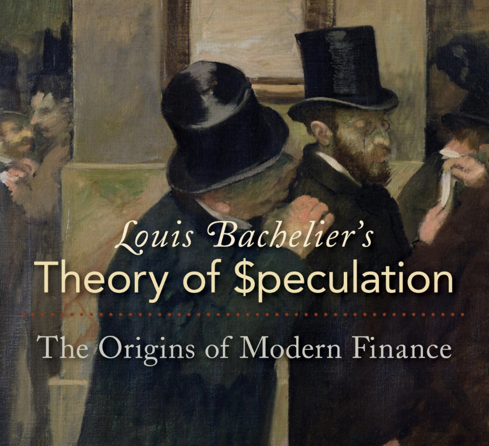
The Arithmetic Brownian model was postulated by Louis Bachelier on his PhD thesis “Theory of Speculation” (1900) as a mathematical model for stock prices movements –known today as the Bachelier model.

One early criticism of the Bachelier model is that the probability distribution which he chose to use to describe stock prices allowed for negative prices. His doctoral dissertation was graded down because of that feature. Today, such feature has became an advantage of the model!

On April 8, 2020, the CME Group posted the note CME Clearing Plan to Address the Potential of a Negative Underlying in Certain Energy Options Contracts,[1] saying that after a threshold on price, it would change its standard energy options model from one based on Geometric Brownian Motion and the Black–Scholes model to the Bachelier model.

Day 5: Arithmetic Brownian Motion

Contents

Day 5: Arithmetic Brownian Motion#

Definition#

🔔 Random Facts 🔔#

More to Read#