Day 4: Brownian Motion#

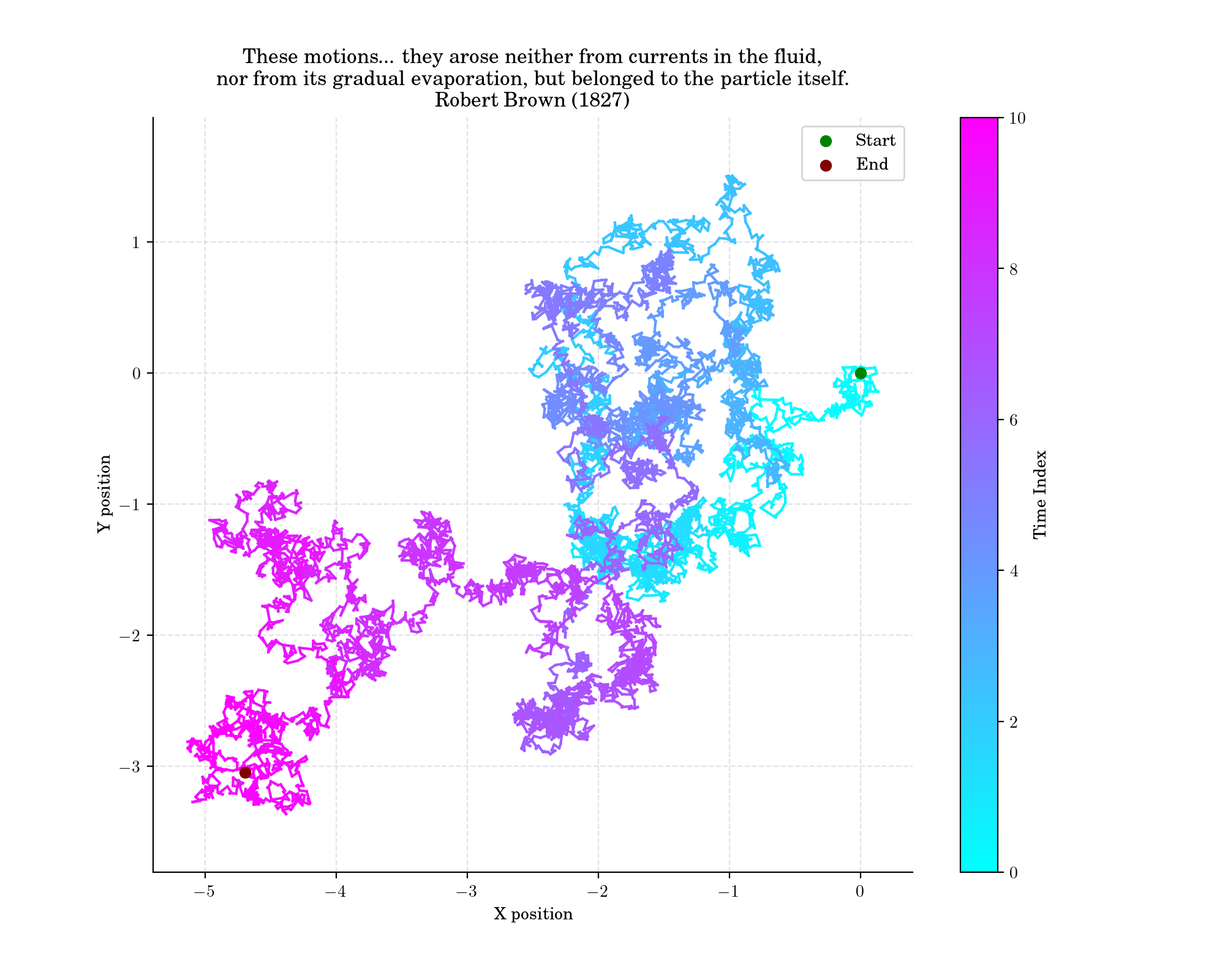
Brownian motion or Brownian movement generally refers to the random motion of particles suspended in a medium (a liquid or a gas). It is named after the Scottish botanist Robert Brown, who first described the phenomenon in 1827, while looking through a microscope at pollen of the plant Clarkia pulchella immersed in water. He saw something like this:

In mathematics, Brownian motion is described by the Wiener process, a continuous-time stochastic process named after American computer scientist, mathematician, and philosopher Norbert Wiener. It is probably the most well-known Lévy processes (càdlàg stochastic processes with stationary independent increments) since occurs frequently in pure and applied mathematics, economics and physics.

Definition#

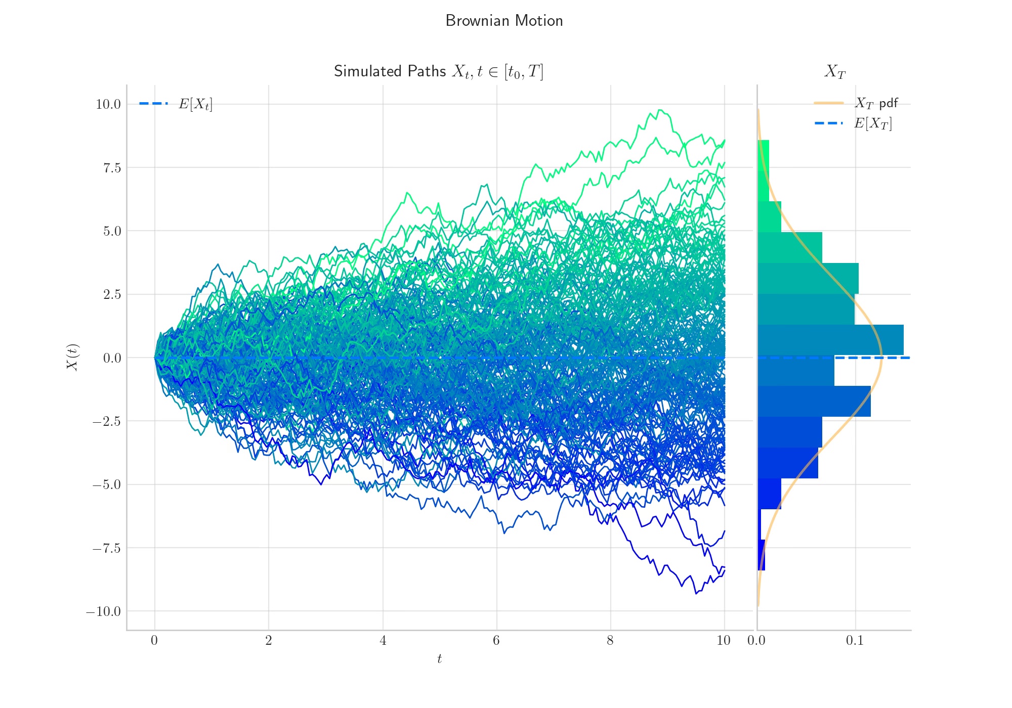
A standard (one dimensional) Wiener process (or Brownian motion) is a stochastic process \(W =\{W(t), t\geq 0\},\) characterised by the following four properties:

1. \(W(0) = 0\)

2. \(W(t)-W(s) \sim N(0, t-s),\) for any \(0\leq s \leq t\)

3. \(W\) has independent increments

4. \(W\) is almost surely continuous.

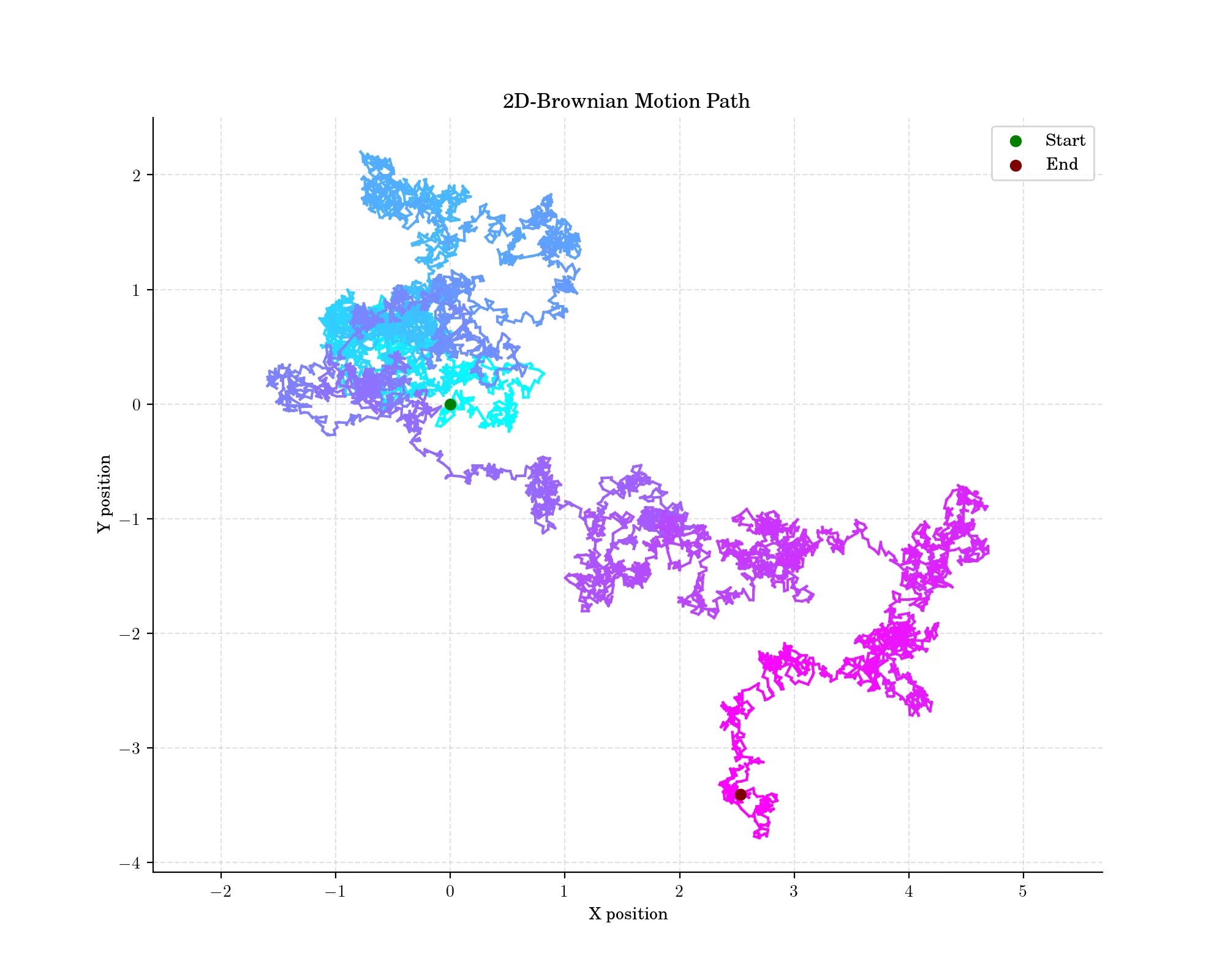
A standard d−dimensional Wiener process is a vector-valued stochastic process defined as

\[W(t) = (W_1(t) ,W_2(t), \cdots, W_d(t)), \qquad t\geq 0,\]

whose components \(W_i\) are independent, standard one-dimensional Wiener processes.

🔔 Random Facts 🔔#

In 1905, Albert Einstein’s published Investigations on the Theory of Brownian Movement a groundbreaking work that provided a deep theoretical explanation of Brownian motion. He developed a mathematical framework linking the seemingly random motion of particles to the kinetic theory of heat, thereby confirming the existence of atoms and molecules as physical entities. He derived an expression that related the diffusion coefficient of particles to measurable properties such as temperature, viscosity, and particle size, enabling experimental validation.

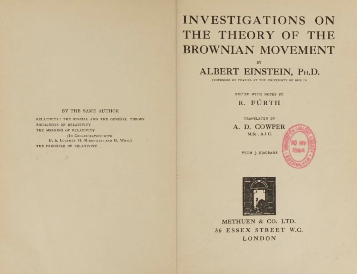
This image has an empty alt attribute; its file name is tempImageeAsG3y.jpg

A copy of the original books is available online and you can even buy a modern edition on Amazon!

In 1923, Norbert Wiener formally proved the existence of the Wiener process. Its mathematical framework indirectly influenced Richard Feynman’s path integral formulation of quantum mechanics. The Wiener process provides a probabilistic foundation for simulating quantum particle paths, as the sum over all possible paths in Feynman’s formulation is conceptually akin to the summation over random Brownian trajectories.
The Wiener process can be constructed as the scaling limit of a Random Walk. This is known as Donsker’s theorem. Check out my previous post about this construction.
Like the Random Walk, the Wiener process is recurrent in one or two dimensions (meaning that it returns almost surely to any fixed neighborhood of the origin infinitely often) whereas it is not recurrent in dimensions three and higher.
The Brownian motion, has significant applications in finance, tracing back to French mathematician Louis Bachelier’s pioneering 1900 thesis, Theory of Speculation. Bachelier was the first to apply the mathematics of Brownian motion to model stock price movements, preceding Einstein’s formalisation of the phenomenon. His work introduced the concept of price fluctuations as a random walk, laying the foundation for modern financial mathematics. Today, the Wiener process is a key component of models like the Black-Scholes equation for option pricing and is used extensively to model asset prices, interest rates, and risk in stochastic calculus frameworks.

Day 4: Brownian Motion

Contents

Day 4: Brownian Motion#

Definition#

🔔 Random Facts 🔔#

More to Read#