Day 19: Zeta

• 
• 

/home/runner/work/advent-calendar-2023/advent-calendar-2023/bonus/plot_advent_19_Zeta_Bonus.py:28: SyntaxWarning: invalid escape sequence '\R'
  plt.plot(ys, real_parts, label="$\Re[\zeta(\\frac{1}{2} + i y)]$")
/home/runner/work/advent-calendar-2023/advent-calendar-2023/bonus/plot_advent_19_Zeta_Bonus.py:29: SyntaxWarning: invalid escape sequence '\I'
  plt.plot(ys, imag_parts, label="$\Im[\zeta(\\frac{1}{2} + i y)]$")
/home/runner/work/advent-calendar-2023/advent-calendar-2023/bonus/plot_advent_19_Zeta_Bonus.py:30: SyntaxWarning: invalid escape sequence '\z'
  plt.title("Riemann zeta function along the critical line \n  $\zeta(\\frac{1}{2} + i y)$")
/home/runner/work/advent-calendar-2023/advent-calendar-2023/bonus/plot_advent_19_Zeta_Bonus.py:59: SyntaxWarning: invalid escape sequence '\z'
  plt.title("Riemann zeta function along the critical line \n  $\zeta(\\frac{1}{2} + i y)$")
/home/runner/work/advent-calendar-2023/advent-calendar-2023/bonus/plot_advent_19_Zeta_Bonus.py:60: SyntaxWarning: invalid escape sequence '\R'
  plt.xlabel("$\Re[\zeta(\\frac{1}{2} + i y)]$")
/home/runner/work/advent-calendar-2023/advent-calendar-2023/bonus/plot_advent_19_Zeta_Bonus.py:61: SyntaxWarning: invalid escape sequence '\I'
  plt.ylabel("$\Im[\zeta(\\frac{1}{2} + i y)]$")

# Author: Dialid Santiago <d.santiago@outlook.com>
# License: MIT
# Description: Advent Calendar 2023

import numpy as np
import matplotlib.pyplot as plt
from mpmath import zeta
from matplotlib.collections import LineCollection

plt.style.use("https://raw.githubusercontent.com/quantgirluk/matplotlib-stylesheets/main/quant-pastel-light.mplstyle")

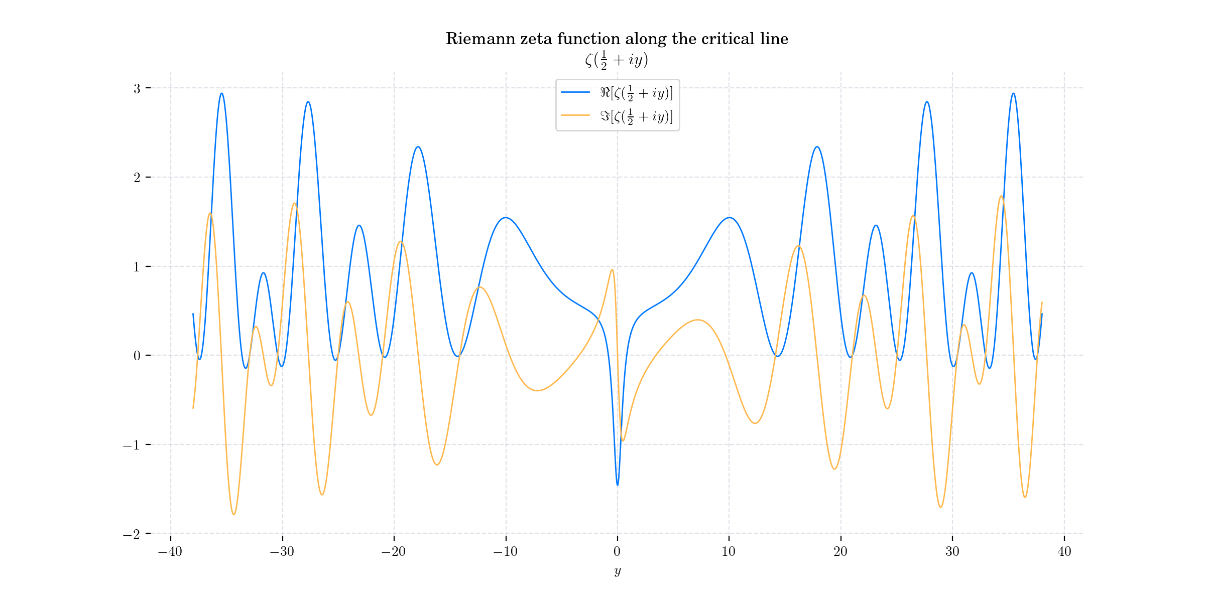
ys = np.linspace(-38, 38, 2000)
zs = [complex(0.5, y) for y in ys]
z_values = [complex(zeta(z)) for z in zs]

real_parts = [zv.real for zv in z_values]
imag_parts = [zv.imag for zv in z_values]

fig = plt.figure(figsize=(12, 6))
plt.plot(ys, real_parts, label="$\Re[\zeta(\\frac{1}{2} + i y)]$")
plt.plot(ys, imag_parts, label="$\Im[\zeta(\\frac{1}{2} + i y)]$")
plt.title("Riemann zeta function along the critical line \n  $\zeta(\\frac{1}{2} + i y)$")
plt.xlabel("$y$")
plt.legend()
plt.box(on=False)
fig.savefig('19_Zeta_Bonus1')
plt.show()

x = np.array(real_parts)
y = np.array(imag_parts)
dydx = ys
# Create a set of line segments so that we can color them individually
# This creates the points as an N x 1 x 2 array so that we can stack points
# together easily to get the segments. The segments array for line collection
# needs to be (numlines) x (points per line) x 2 (for x and y)
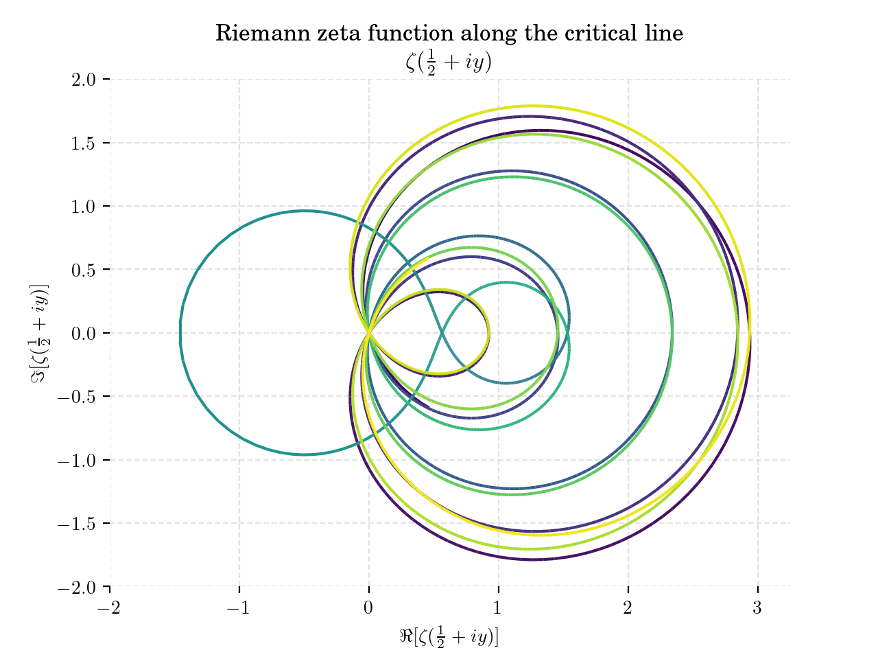
points = np.array([x, y]).T.reshape(-1, 1, 2)
segments = np.concatenate([points[:-1], points[1:]], axis=1)

fig, axs = plt.subplots(1, 1)

# Create a continuous norm to map from data points to colors
norm = plt.Normalize(dydx.min(), dydx.max())
lc = LineCollection(segments, cmap='viridis', norm=norm)
# Set the values used for color mapping
lc.set_array(dydx)
lc.set_linewidth(1.5)
line = axs.add_collection(lc)
axs.set_xlim(-2, 3.25)
axs.set_ylim(-2, 2)

plt.title("Riemann zeta function along the critical line \n  $\zeta(\\frac{1}{2} + i y)$")
plt.xlabel("$\Re[\zeta(\\frac{1}{2} + i y)]$")
plt.ylabel("$\Im[\zeta(\\frac{1}{2} + i y)]$")
plt.box(on=False)
# fig.savefig('19_Zeta_Bonus2')
plt.show()