Day 19 : Zeta

The zeta distribution is a discrete probability distribution with support on \(\mathbb{N^+}\) and is defined by a shape parameter \(s>1\). As its name indicates, it is closely related to the famous Riemann zeta function 𝜁, named after German mathematician Bernhard Riemann.

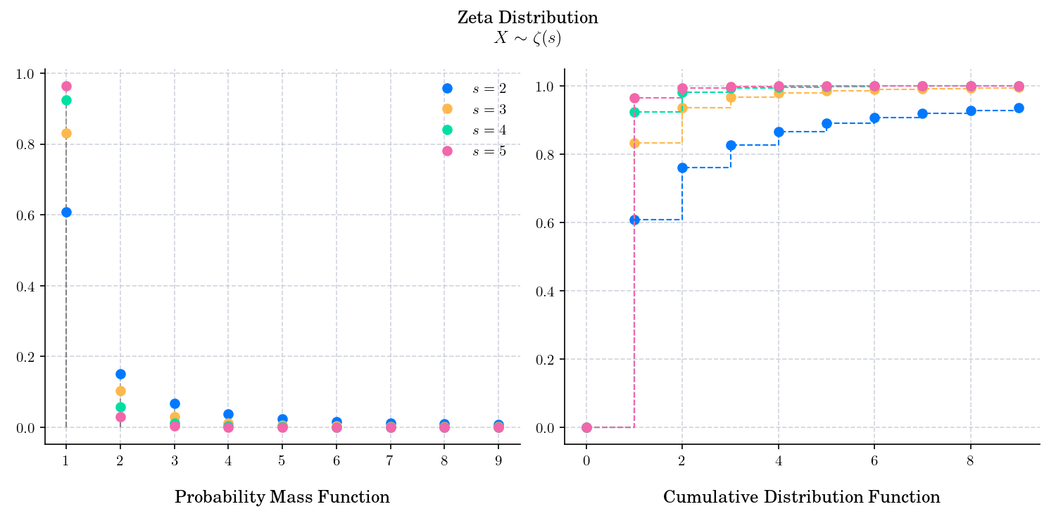
The probability mass function is given by

\[f(k) = \frac{1}{\zeta(s) k^s}, \qquad k = 1, 2, 3, \cdots.\]

The cumulative distribution function is given by

\[F(k) =\frac{H_{k, s}}{\zeta(s)},\]

where \(H_{k, s}\) is the generalized harmonic number:

\[H_{k,s} = \sum_{i=1}^k \frac{1}{i^s}.\]

🔔 Random Facts 🔔

• It is used to model the size or ranks of certain types of objects randomly chosen from certain types of populations. Typical examples include the frequency of occurrence of a word randomly chosen from a text, or the population rank of a city randomly chosen from a country.

• It is also known as the Zipf distribution, in honor of American linguist and philologist George Zipf, who studied statistical occurrences in different languages.

• The n-th raw moment of the zeta distribution with parameter \(s\), is defined as:

\[m_{n}=E(X^{n})={\frac {1}{\zeta (s)}}\sum _{{k=1}}^{\infty }{\frac {1}{k^{{s-n}}}}\]

The series on the right is just a series representation of the Riemann zeta function, but it only converges for values of \(s-n\) that are greater than unity. Thus,

The ratio of the zeta functions is well-defined, even for n > s − 1 because the series representation of the zeta function can be analytically continued. This does not change the fact that the moments are specified by the series itself, and are therefore undefined for large n. Therefore, the moment generating function of the zeta distribution does not exist.

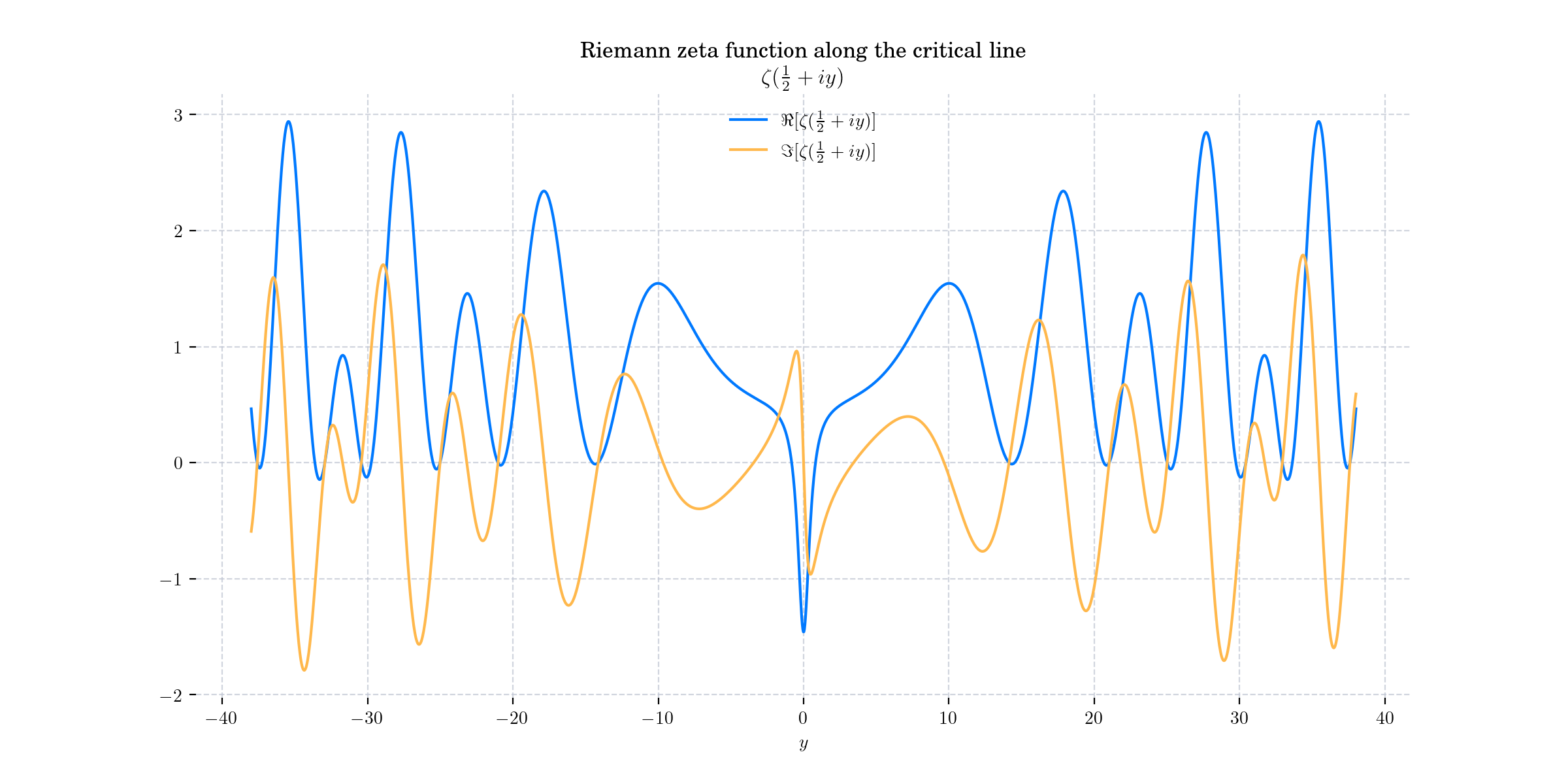
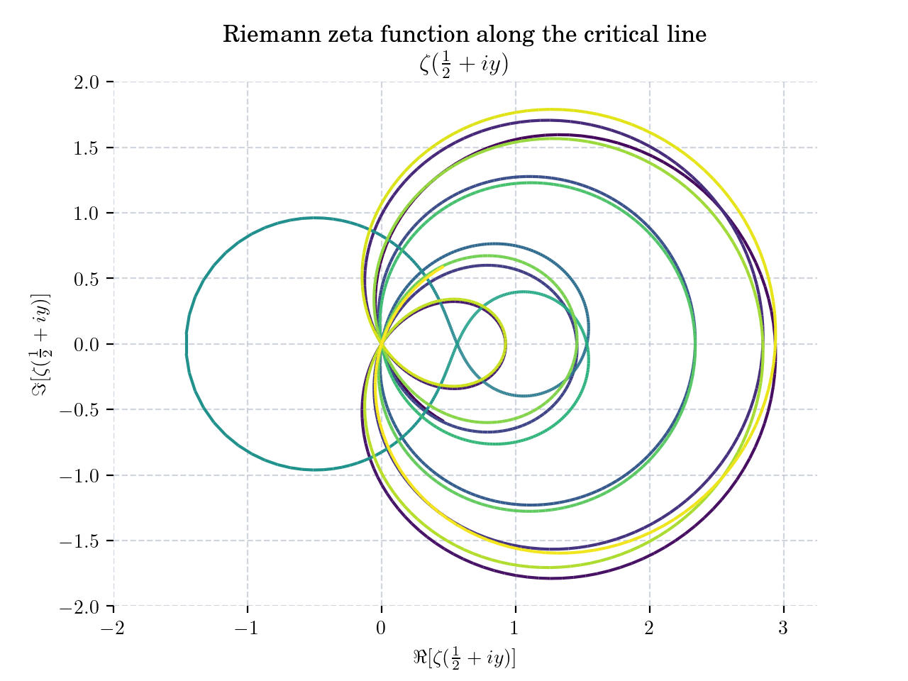
Today’s bonus is two plots of the Riemann Zeta function evaluated in the critical line!