Day 3 : Cauchy

The Cauchy distribution, named after French mathematician Augustin Cauchy, and also called the Lorentzian distribution or Lorentz distribution, is a continuous distribution describing resonance behaviour.

The Cauchy distribution with location and scale parameters \(x_0\) and \(\gamma\), respectively, describes the distribution of the x-intercept of a ray issuing from \((x_{0},\gamma)\) with a uniformly distributed angle. The Cauchy distribution is often used in statistics as the canonical example of a “pathological” distribution since both its expected value and its variance are undefined.

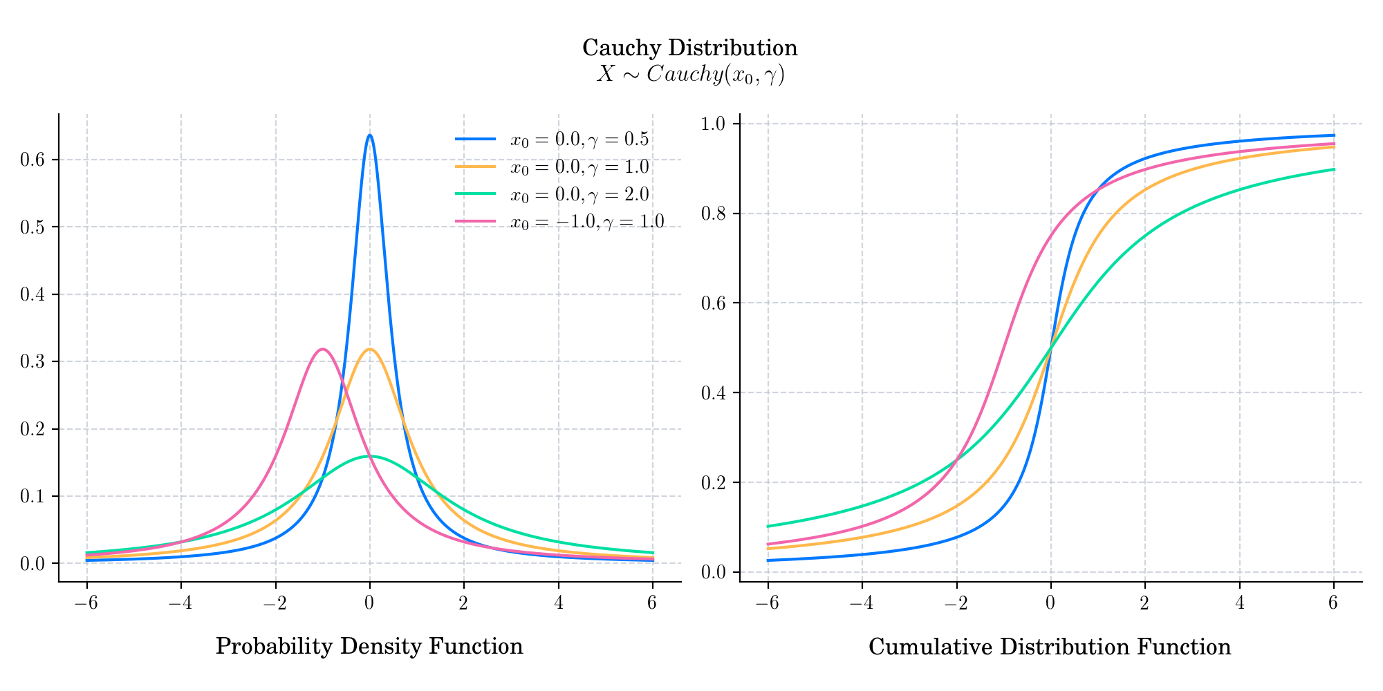
The probability density function is given by

\[f(x) = \frac{1}{\pi \gamma \left[ 1 + \left(\frac{x-x\_0}{\gamma} \right)^2 \right]}, \qquad x\in(-\infty, \infty).\]

The cumulative distribution function is given by

\[F(x) = \frac{1}{\pi} \arctan \left(\frac{x-x\_0}{\gamma}\right) +\frac{1}{2}, \qquad x\in(-\infty, \infty).\]

🔔 Random Facts 🔔

• Let \(X\) and \(Y\) be independent standard normal distributions \(X, Y \sim N(0, 1)\). Their ratio follows a standard (location and scale parameters equal to 0 and 1, respectively) Cauchy distributions X/Y ~ Cauchy(0,1)

• The Cauchy distribution is stable 🪄. Moreover, it is one of the few stable distributions with a probability density function that can be expressed analytically, the others being the normal distribution and the Lévy distribution