Day 8 : Hypergeometric

The hypergeometric distribution is a discrete probability distribution that describes the probability of \(k\) successes (random draws for which the object drawn has a specified feature) in \(n\) draws, without replacement, from a finite population of size \(N\) that contains exactly \(K\) objects with that feature, wherein each draw is either a success or a failure.

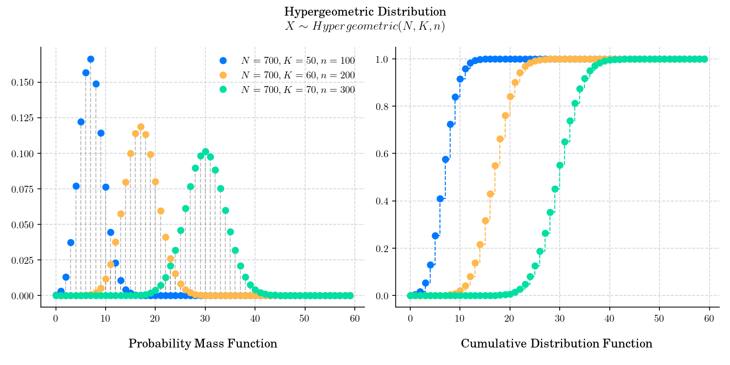
The probability mass function is given by

\[f(k) =\frac{ {K \choose k}{ N-K \choose n-k} }{ N \choose n }.\]

The cumulative distribution function is given by

\[F(k) = \frac{ {n \choose k+1}{ N-n \choose K-k-1} }{ N \choose K } {_3}{F}{_2}(1, k+1-K, k+1-n; k+2, N+k+2-K-n; 1),\]

where \({_2}F_{_1}\) is the generalised hypergeometric function.

🔔 Random Facts 🔔

• Similarly to the Binomial distribution, it describes the probability of successes in a given number of draws. The difference is that there is no replacement after each draw.

• Quality control in manufacturing is a common application of the Hypergeometric Distribution. It is used by engineers and quality experts to test a sample of products from an assembly line to identify defective items.

• The name Hypergeometric is relatively recent but the distribution first appears as the solution to Problem IV of Huygens’s De Ratiociniis in Ludo Aleae (1657, p. 12) (“The Value of all Chances in Games of Fortune”). Several people, besides Christiaan Huygens, solved the problem and James Bernoulli and de Moivre gave solutions for the general case. See Hald (1990, pp. 201-2). At the end of the 19th century Karl Pearson wrote a paper in which he considered fitting the distribution (given by the “hypergeometrical series”) to data: “On Certain Properties of the Hypergeometrical Series, and on the Fitting of such Series to Observation Polygons in the Theory of Chance” Philosophical Magazine, 47, (1899), 236-246.