Day 10 : Laplace

The Laplace distribution is a continuous probability distribution named after French mathematician Pierre-Simon Laplace. It is sometimes called the double exponential distribution, because it looks like two exponential distributions spliced together back-to-back. The Laplace distribution is defined by a location parameter \(\mu\in\mathbb{R}\) and a scale parameter \(b>0\), which is sometimes referred as “diversity”. It has support \((-\infty, \infty)\) and is symmetric around its location parameter \(\mu\).

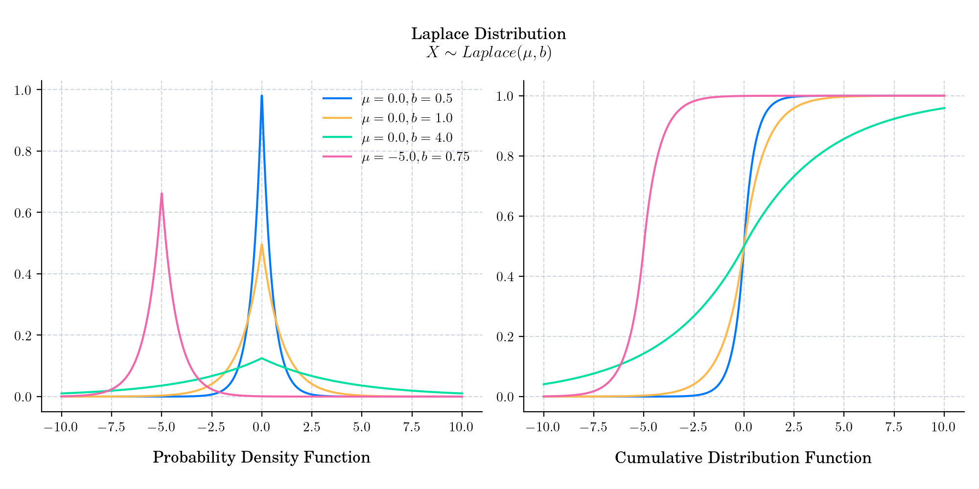
The probability density function is given by

\[f(x) =\frac{1}{2b}\exp\left( -\frac{|x-\mu|}{b} \right).\]

The cumulative distribution function is given by

\[\begin{split}F(x) = \begin{cases} \frac{1}{2} \exp\left(\frac{x-\mu}{b} \right) & \hbox{if } x\leq \mu\\ 1 - \frac{1}{2} \exp\left(-\frac{x-\mu}{b} \right) & \hbox{if } x\geq \mu\end{cases}.\end{split}\]

🔔 Random Facts 🔔

• The Laplace distribution is often referred to as “Laplace’s first law of errors”. Laplace published it in 1774, modeling the frequency of an error as an exponential function of its magnitude once its sign was disregarded. Laplace would later replace this model with his “second law of errors”, based on the normal distribution, after the discovery of the central limit theorem.

• If \(X, Y \sim Exponential(\lambda)\), then \(X-Y\sim Laplace(0, 1/\lambda)\).

• Just as ridge regression can be interpreted as linear regression for which the coefficients have been assigned normal prior distributions, lasso (least absolute shrinkage and selection operator; also Lasso or LASSO) can be interpreted as linear regression for which the coefficients have Laplace prior distributions.