Day 14 : Lognormal

A lognormal distribution is a continuous probability distribution of a random variable whose logarithm is normally distributed. Thus, if the random variable X is log-normally distributed, then Y = ln(X) has a normal distribution. Equivalently, if Y has a normal distribution, then the exponential function of Y, X = exp(Y) , has a log-normal distribution.

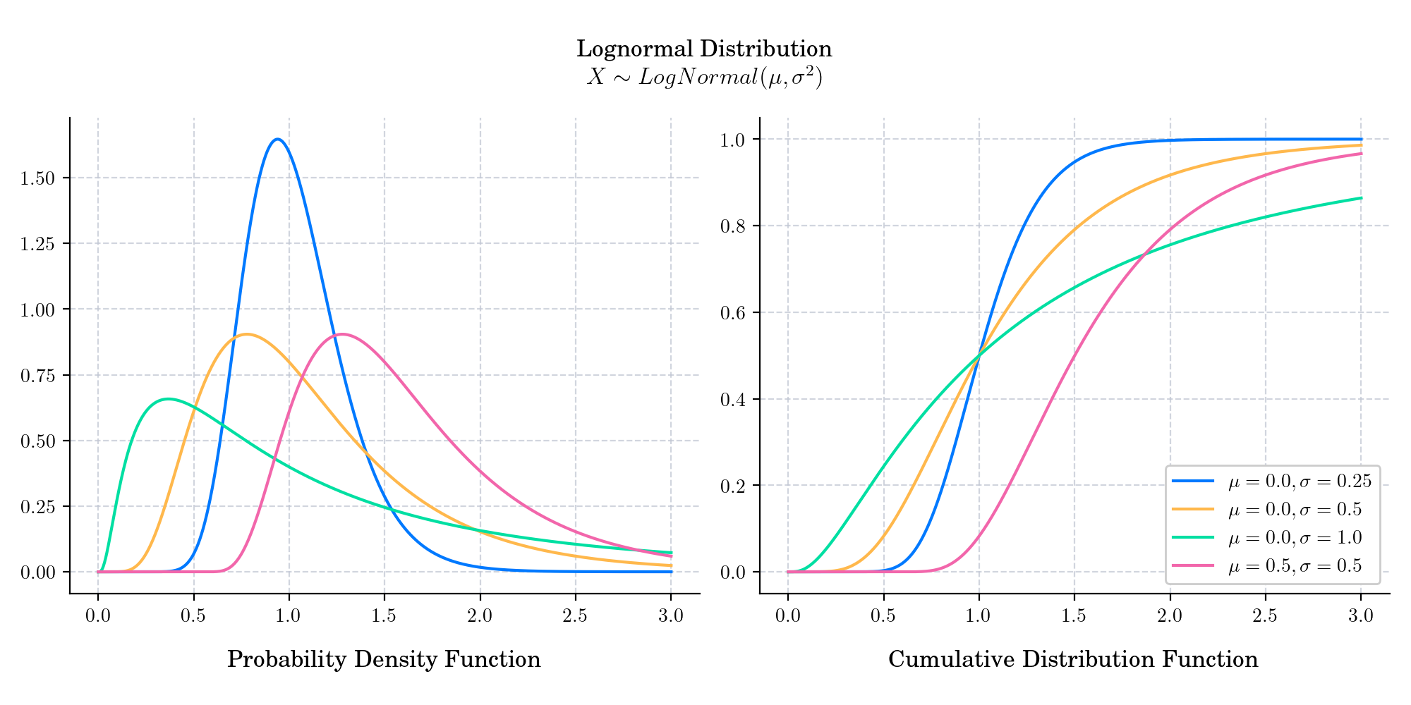
The probability density function is given by

\[f(x) = \frac{1}{x\sigma\sqrt{2\pi}} \exp\left(- \frac{ (\ln x - \mu)^2 }{2\sigma^2} \right) \qquad x\geq 0.\]

The cumulative distribution function is given by

\[F(x) = \frac{1}{2}\left[ 1+ \hbox{erf} \left( \frac{ \ln x - \mu }{\sigma \sqrt{2} } \right) \right] =\Phi\left( \frac{ \ln(x) - \mu }{2\sigma^2} \right) , \qquad x\geq 0,\]

where erf is the complementary error function, and \(\Phi\) is the cdf of a standard normal distribution.

🔔 Random Facts 🔔

• The lognormal distribution is due to the works of Galton, F. (The geometric mean in vital and social statistics, 1879) and McAlister, D. (The law of the geometric mean, 1879) who obtained expressions for the mean, median, mode, variance, and certain quantiles of the resulting distribution. You can find digital copies of the original manuscripts here!

• It is used extensively in reliability applications to model failure times. Indeed, the lognormal and the Weibull distributions are probably the most commonly used distributions in reliability applications.

• Finally, the lognormal distribution is extensively used in Finance. In particular, the famous Black and Scholes models relies on the assumption that the stock price follows a geometric Brownian motion. This means that the marginal densities of the stock price follow a log-normal distribution.