Compound Effect

• 
• 

# Author: Dialid Santiago <d.santiago@outlook.com>
# License: MIT
# Description: Advent Calendar 2025 - Plot Compound Effect


import numpy as np
import matplotlib.pyplot as plt

plt.style.use("https://raw.githubusercontent.com/quantgirluk/matplotlib-stylesheets/main/quant-pastel-light.mplstyle")

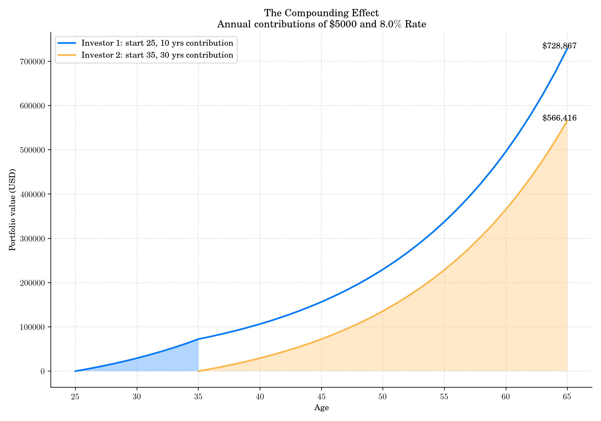
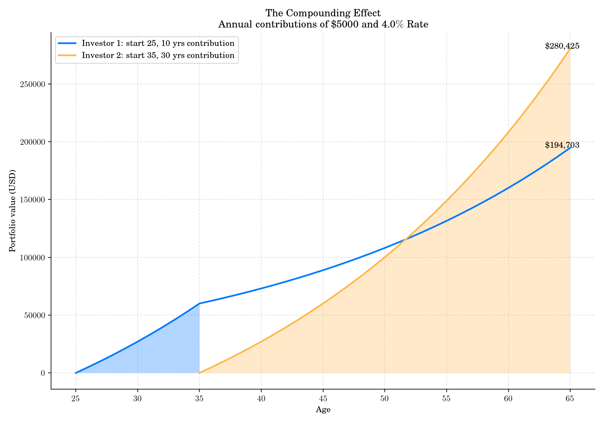
def plot_compound_effect(r=0.08, start1=25, start2=35, end_age=65, n1=10, annual_contrib=5000):


    # Contribution periods
    years1 = np.arange(0, end_age - start1 + 1)
    years2 = np.arange(0, end_age - start2 + 1)

    def fv_series(contrib, r, n_years):
        final = contrib * (1-(1 + r)**(n_years))*(1./(-r))
        return final

    # Investor 1: n1 years of contributions from start1 and then compounding only until end_age
    fv1 = fv_series(annual_contrib, r, n1)
    balance1 = np.concatenate([
        [fv_series(annual_contrib, r, t) for t in range(0, n1+1)],
        fv1 * (1 + r)**np.arange(1, end_age - (start1 + n1) + 1)
    ])

    # Investor 2: contributes from start2 until end_age
    n2 = end_age - start2
    balance2 = np.array([fv_series(annual_contrib, r, t) for t in range(0, n2+1)])

    # Ages
    ages1 = np.arange(start1, end_age + 1)
    ages2 = np.arange(start2, end_age + 1)


    fig = plt.figure(figsize=(10,7), dpi=200)

    # Plot lines
    plt.plot(ages1, balance1, label=f'Investor 1: start {start1}, 10 yrs contribution', linewidth=2)
    plt.plot(ages2, balance2, label=f'Investor 2: start {start2}, 30 yrs contribution', linewidth=2)

    # Shaded areas
    plt.fill_between(ages1[:n1+1], balance1[:n1+1], alpha=0.3)
    plt.fill_between(ages2, balance2, alpha=0.3)

    # Final value labels
    plt.annotate(f"\\${balance1[-1]:,.0f}", (ages1[-1], balance1[-1]), xytext=(ages1[-1]-2, balance1[-1]*1.))
    plt.annotate(f"\\${balance2[-1]:,.0f}", (ages2[-1], balance2[-1]), xytext=(ages2[-1]-2, balance2[-1]*1.))

    plt.xlabel('Age')
    plt.ylabel('Portfolio value (USD)')
    plt.title(f"The Compounding Effect \n Annual contributions of \\${annual_contrib} and {r*100}$\\%$ Rate")
    plt.legend()
    plt.grid(True)
    plt.tight_layout()
    plt.show()

    return fig


case1 = plot_compound_effect(r=0.08, start1=25, start2=35, end_age=65, n1=10, annual_contrib=5000)

case2 = plot_compound_effect(r=0.04, start1=25, start2=35, end_age=65, n1=10, annual_contrib=5000)