Day 10: Correlation#
“One of the first things taught in introductory statistics textbooks is that correlation is not causation. It is also one of the first things forgotten”
—Thomas Sowell, The Vision of the Anointed (1995)
Correlation is a statistical measure that describes the strength and direction of a relationship between two variables. It quantifies how changes in one variable are associated with changes in another variable.
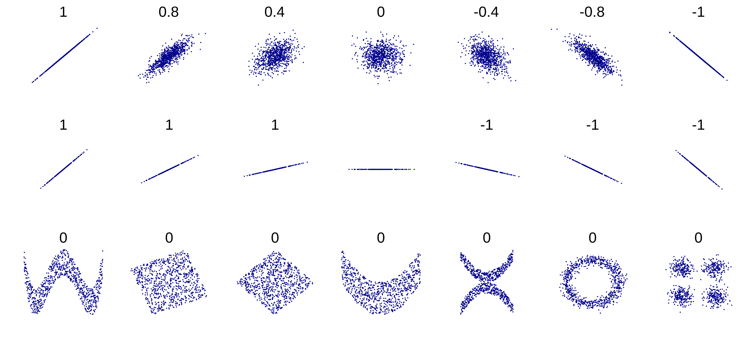
The image above shows several sets of (x, y) points, with the Pearson correlation coefficient of x and y for each set. The correlation reflects the noisiness and direction of a linear relationship (top row), but not the slope of that relationship (middle), nor many aspects of nonlinear relationships (bottom). N.B.: the figure in the center has a slope of 0 but in that case, the correlation coefficient is undefined because the variance of Y is zero.
Pearson Correlation Coefficient#
Definition. The most common measure of correlation is the Pearson correlation coefficient, denoted by \(\rho\). It measures linear correlation between two sets of data. It is the ratio between the covariance of two variables and the product of their standard deviations; thus, it is essentially a normalized measurement of the covariance, such that the result always has a value between −1 and 1
It is calculated using the formula:
where
\(X_i\) and \(Y_i\) are the individual data points,
\(\bar{X}\) and \(\bar{Y}\) are
the means of the variables X and Y, respectively.
The Pearson correlation coefficient does not have units, allowing comparison of the strength of the joint association between different pairs of random variables that do not necessarily have the same units.
Spearman’s Rank Correlation Coefficient#
Another measure of correlation is Spearman’s rank correlation coefficient, denoted by \(\rho_s\) or \(r_s\). It assesses how well the relationship between two variables can be described using a monotonic function.
The Spearman correlation coefficient is defined as the Pearson correlation coefficient between the rank variables.
If all \(n\) ranks are distinct integers, i.e. there are no ties, the Spearman correlation coefficient can be calculated using the formula:
where - \(d_i\) is the difference between the ranks of corresponding values of the two variables, - \(n\) is the number of data points.
Spearman’s rank correlation coefficient is a non-parametric, meaning it does not assume a specific distribution for the data, measure.
Kendall’s Tau Coefficient#
Kendall’s tau coefficient, denoted by \(\tau\), is another non-parametric measure of correlation that assesses the strength and direction of association between two variables. It is based on the concept of concordant and discordant pairs of observations.
It is calculated using the formula:
where
\(C\) is the number of concordant pairs,
\(D\) is the number of discordant pairs,
\(n\) is the number of data pairs.
Visualizing Correlation#
Scatter plots are a common way to visualize correlation between two variables. Here are some examples of different correlation scenarios:
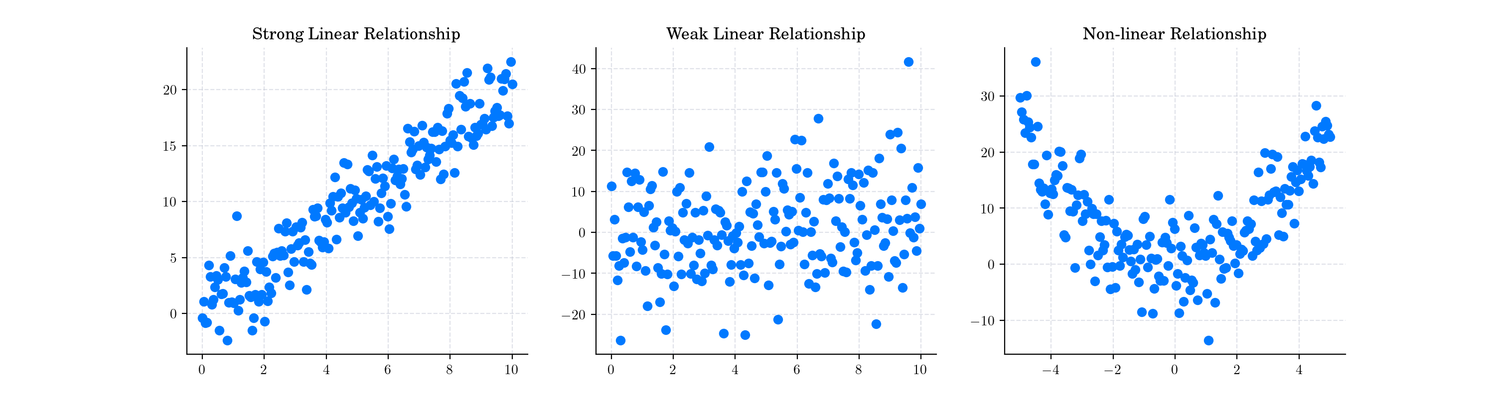
Correlation Examples#
- Strong Linear data
Pearson Correlation: 0.9452991322773132
Spearman Correlation: 0.9503532588314709
Kendall Tau: 0.7990954773869346
- Weak linear data
Pearson Correlation: 0.1950766195754882
Spearman Correlation: 0.16760219005475138
Kendall Tau: 0.11125628140703517
- Non-linear quadratic data
Pearson Correlation: 0.007220503653477844
Spearman Correlation: 0.029063226580664524
Kendall Tau: 0.024623115577889446
In the case of multiple variables, correlation matrices are often used to summarize the pairwise correlations between all variables in a dataset. For visualizations, heatmaps and correlograms are commonly employed.
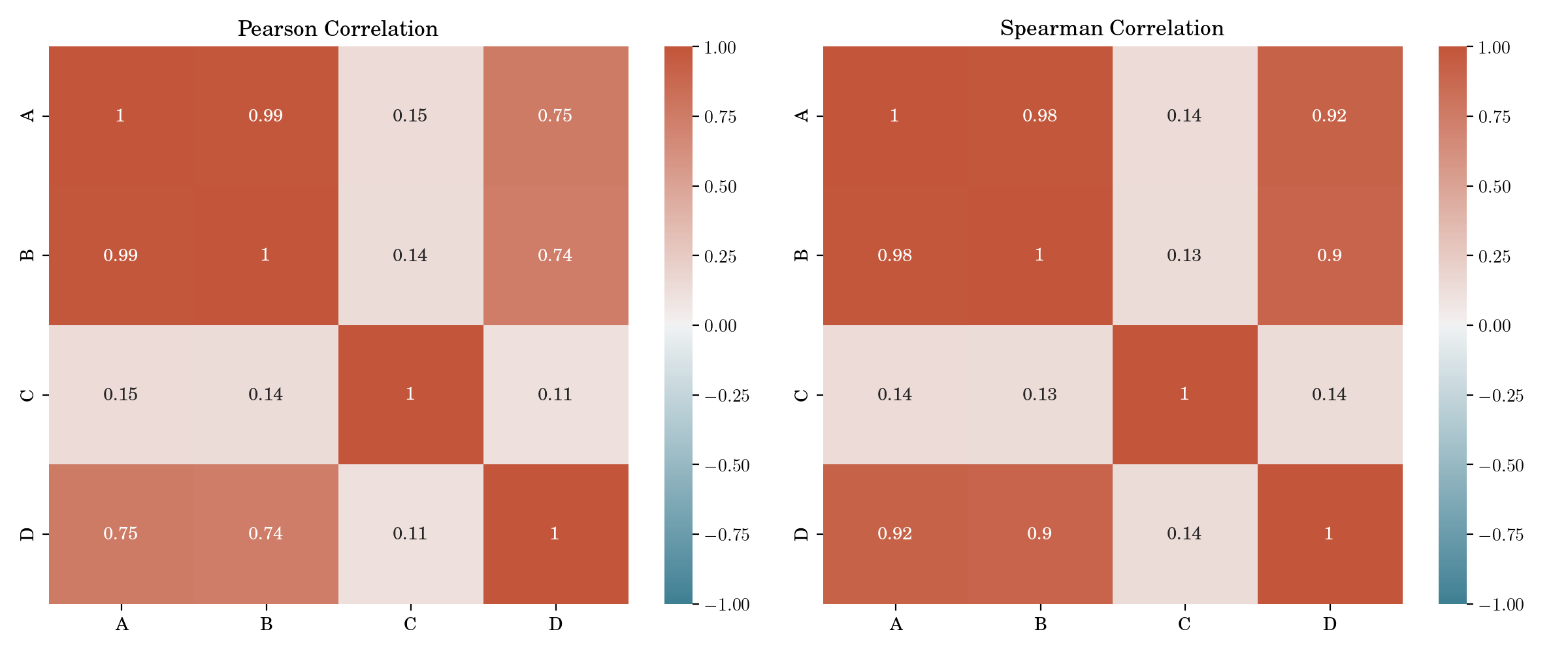
Correlation Matrices and Heatmaps#
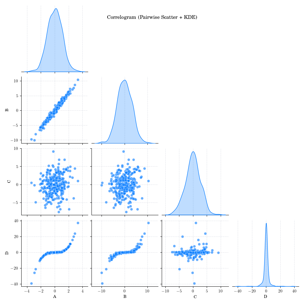
Correlograms showing scatter plots and Kernel Density Estimates (KDE) for all variable pairs.#
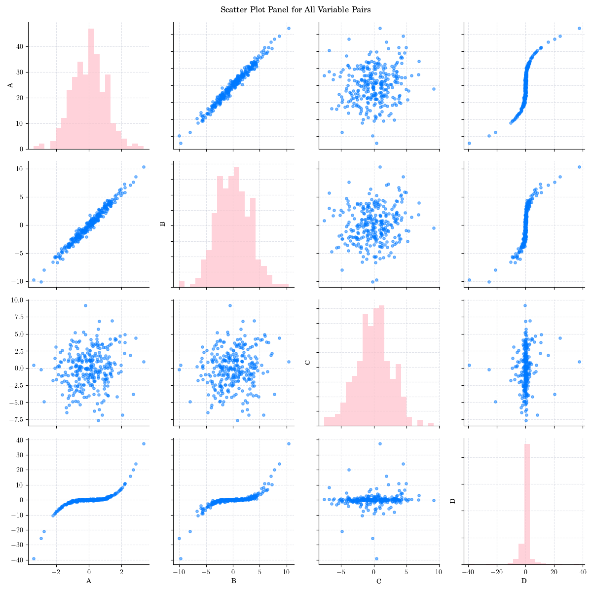
Scatter Plot and Histogram panel for all variable Pairs.#
Random Facts#
Pearson correlation was developed by English biostatistician and mathematician Karl Pearson from a related idea introduced by Francis Galton in the 1880s, and for which the mathematical formula was derived and published by Auguste Bravais in 1844. The naming of the coefficient is thus an example of Stigler’s Law.
Spearman’s rank correlation coefficient was developed by Charles Spearman in 1904. It is based on the earlier work of Francis Galton on rank correlation.
Kendall’s tau coefficient was developed by Maurice Kendall in 1938 as a measure of ordinal association between two quantities. Although Gustav Fechner had proposed a similar measure in the context of time series in 1897.
In finance, correlation is a key concept in portfolio management and risk assessment. Investors use correlation to diversify their portfolios by combining assets that have low or negative correlations, thereby reducing overall risk.