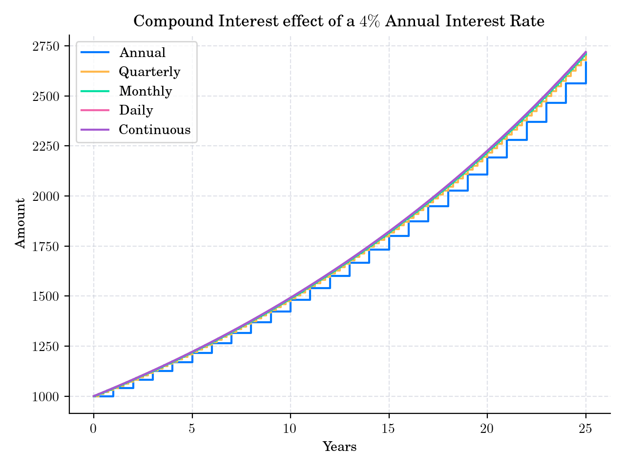
Compounded Interest

# Author: Dialid Santiago <d.santiago@outlook.com>
# License: MIT
# Description: Advent Calendar Day


# Visualisation: step functions approaching continuous compounding
import numpy as np
import matplotlib.pyplot as plt

plt.style.use(
    "https://raw.githubusercontent.com/quantgirluk/matplotlib-stylesheets/main/quant-pastel-light.mplstyle")

P = 1000
r = 0.04  # 4% annual interest
T = 25 # years
times = np.linspace(0, T, 1000)

# Different compounding frequencies: Annual, Quarterly, Monthly, Daily
freqs = [1, 4, 12, 365]
freqs_labels = {1: 'Annual', 4: 'Quarterly', 12: 'Monthly', 365: 'Daily'}
results = {}

for n in freqs:
    # Discrete compounding values at specific periods
    t_points = np.arange(0, T + 1/n, 1/n)
    A = P * (1 + r/n)**(n * t_points)
    results[n] = (t_points, A)

# Continuous compounding
A_cont = P * np.exp(r * times)

plt.figure(dpi=200)

# Plot step functions for discrete compounding
for n, (t_points, A) in results.items():
    plt.step(t_points, A, where='post', label=f'{freqs_labels[n]}', linewidth=1.5)

# Plot continuous compounding
plt.plot(times, A_cont, label='Continuous', linewidth=1.5)

plt.xlabel('Years')
plt.ylabel('Amount')
plt.title(f"Compound Interest effect of a $4\\%$ Annual Interest Rate")
plt.legend()
plt.grid(True)
plt.tight_layout()
plt.show()