Day 5 : Returns

It’s not whether you’re right or wrong, but how much money you make when you’re right and how much you lose when you’re wrong.

—George Soros

When we look at financial time series, there are two common ways to measure the performance of an asset over time, namely linear returns and logarithmic returns.

Definition. Consider an asset that does not pay any intermediate cash income (a zero-coupon bond, such as a Treasury Bill, or a share in a company that pays no dividends). Let \(S_t\) be the price of the security at time \(t\).

The linear or simple return over the time interval \([t, t+ \Delta]\) is defined as

\[R_{t,t+\Delta} = \frac{S_{t+\Delta} - S_t}{S_t} = \frac{S_{t+\Delta}}{S_t} - 1\]

The logarithmic return (also known as continuously compounded return) over the interval \([t, t+\Delta]\) is defined as

\[r_{t,t+\Delta} = \ln\left(\frac{S_{t+\Delta}}{S_t}\right) = \ln(S_{t+\Delta}) - \ln(S_t),\]

and the logarithmic rate of return is given by

\[\rho_{t,t+\Delta} = \frac{r_{t,t+\Delta}}{\Delta} = \frac{1}{\Delta}\ln\left(\frac{S_{t+\Delta}}{S_t}\right).\]

Let’s visualise both time of returns using historical data from daily prices of the S&P 500 Index.

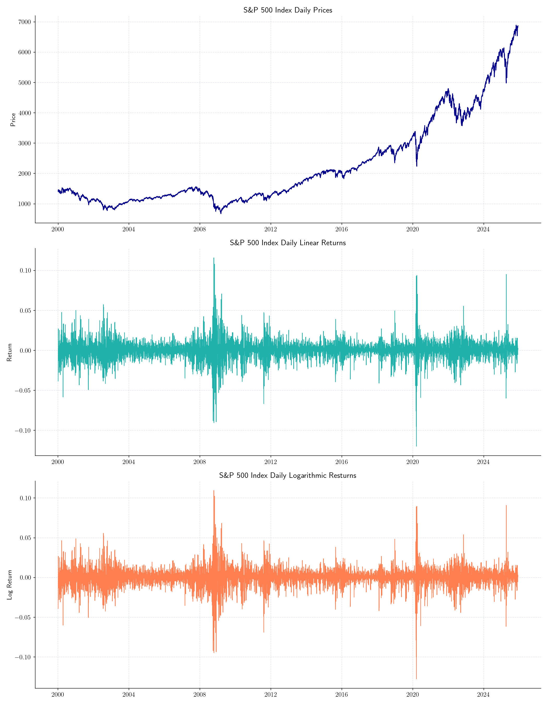
Source: Yahoo Finance.

Logarithmic returns have several advantages over simple returns, including:

• Time Additivity: Log returns can be easily aggregated over multiple periods by summing them up, which is not the case with simple returns

• Symmetry: Log returns treat gains and losses symmetrically, making them more suitable for certain financial models

However, simple returns are more intuitive and easier to understand for many investors, as they directly represent the percentage change in the asset’s price. Both types of returns are widely used in finance, and the choice between them often depends on the specific context and analysis being performed.

In order to visualise the distribution of returns (linear or logarithmic), we can use a histogram or a Box plot.

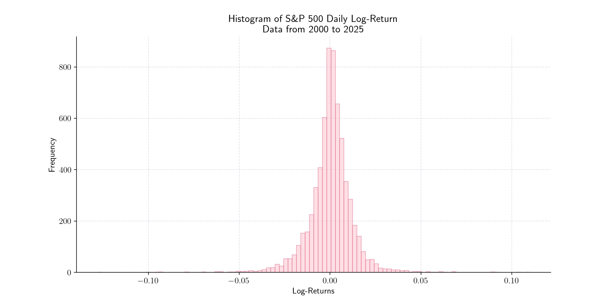
Histogram of Daily Returns of the S&P 500 Index from 2000. Source: Yahoo Finance.

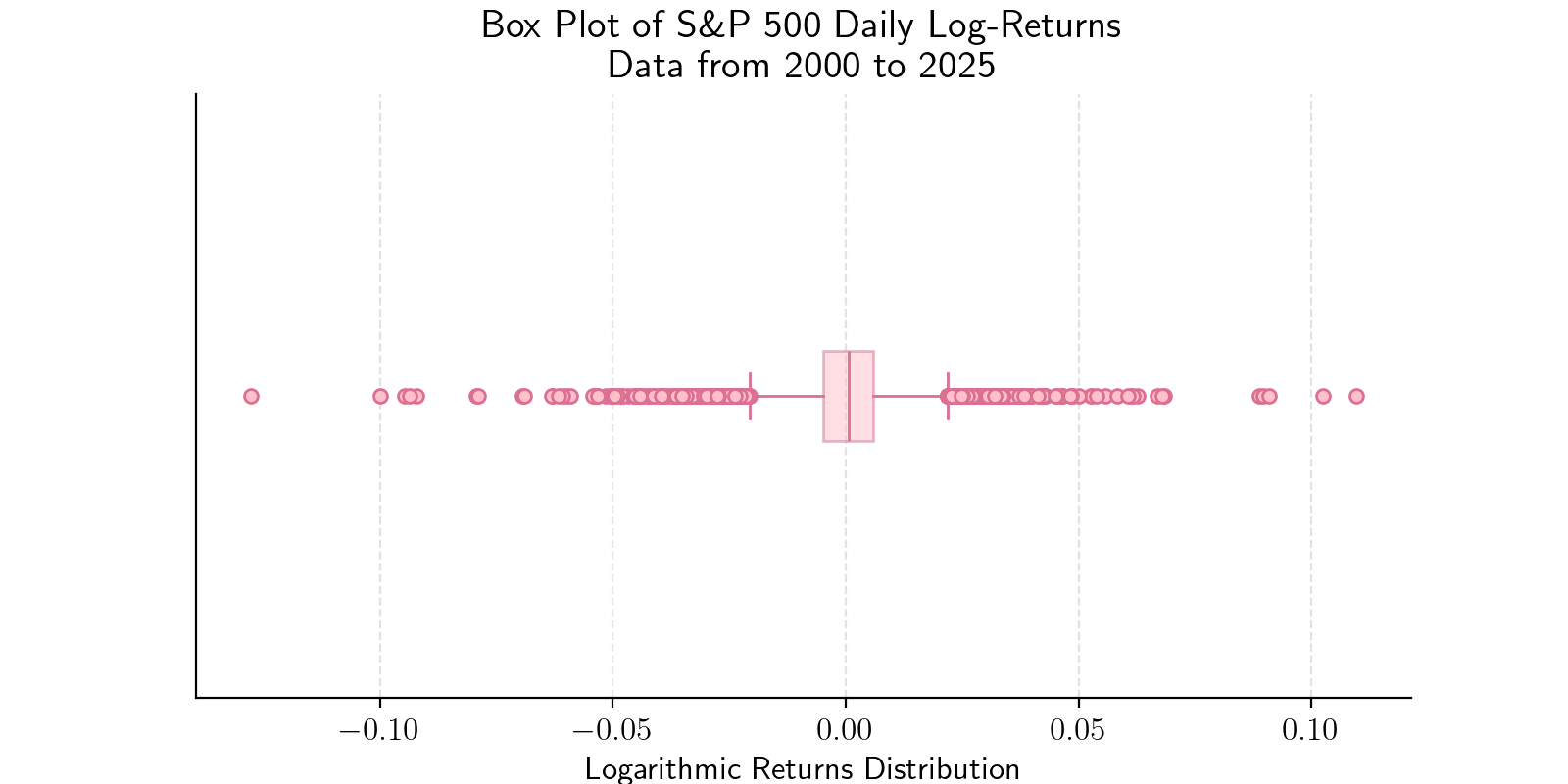
Box Plot of Daily Returns of the S&P 500 Index from 2000. Source: Yahoo Finance.