Day 9 : Exponential Decay#
“The greatest shortcoming of the human race is our inability to understand the exponential function”
—Albert A. Bartlett (1923–2013), Physicist
Exponential decay describes the process of reducing an amount by a consistent percentage rate over a period of time. This concept is widely used in various fields, including physics, biology, and finance, to model phenomena such as radioactive decay, population decline, and depreciation of assets.
Definition. The formula for exponential decay is given by:
where
\(f(t)\) : the quantity at time \(t\),
\(y_0\) : the initial quantity at time \(t = 0\),
\(\lambda\) : the decay constant (a positive number that represents the rate of decay),
\(t\) : time.
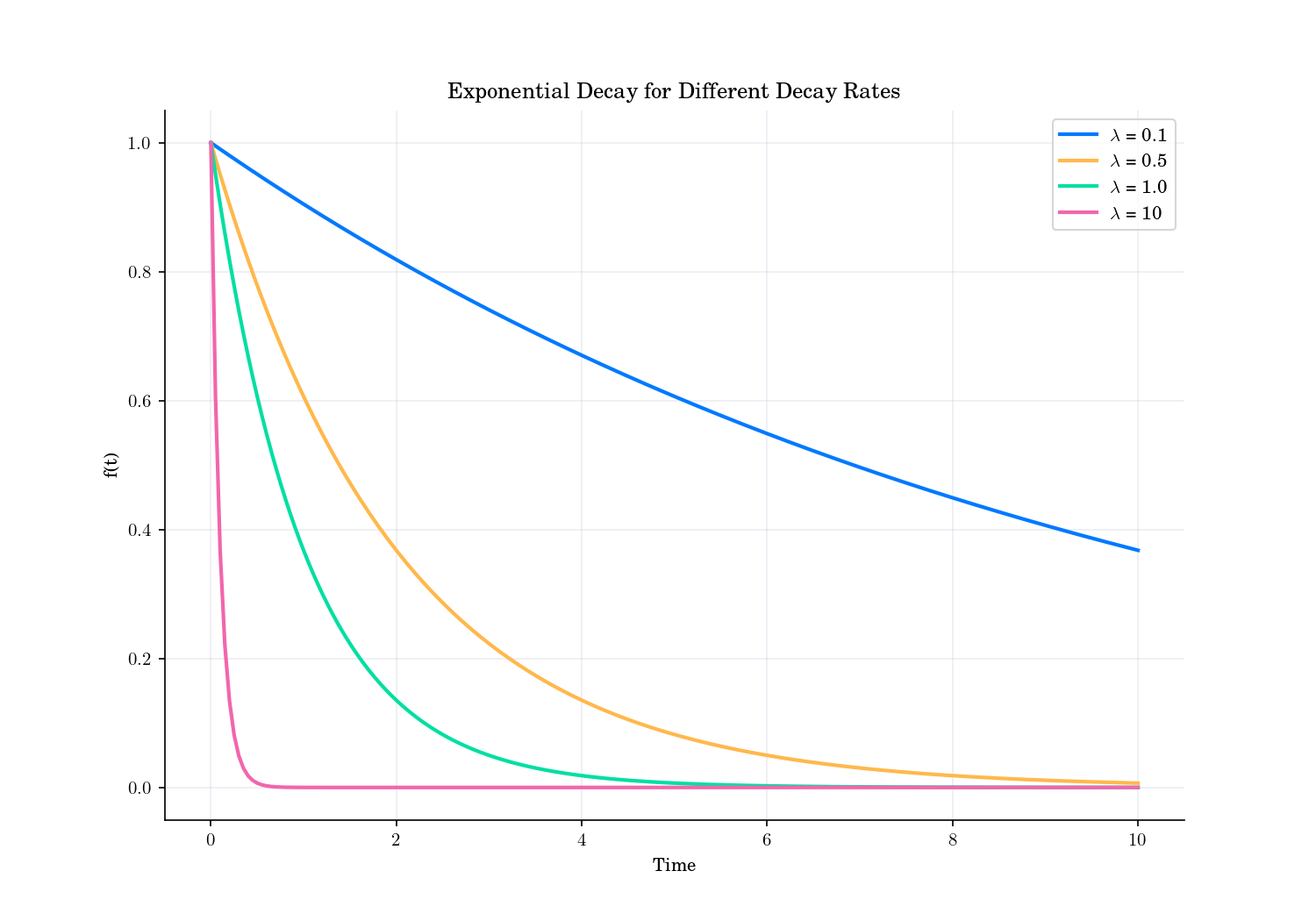
Exponential Decay with different decay rates.#
Two important concepts related to exponential decay are half-life and mean life.
Half-Life: The half-life is the time required for a quantity to reduce to half its initial value. It is related to the decay constant by the formula:
\[t_{1/2} = \frac{\ln(2)}{\lambda}.\]
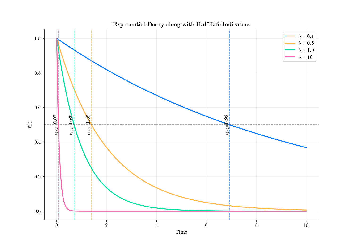
Exponential Decay and Half-life values.#
Mean Life: The mean life is the average time a particle or entity exists before decaying. It is given by:
\[\tau = \frac{1}{\lambda}\]
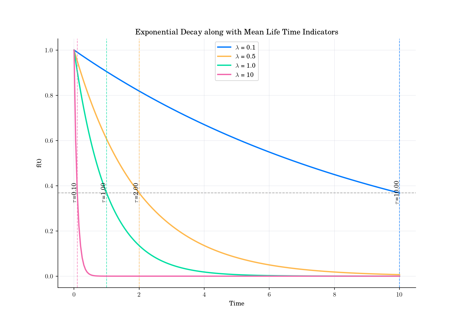
Exponential Decay and Mean Life values.#
Random Facts#
In finance, exponential decay is often used to model the depreciation of assets, where the value of an asset decreases over time at a rate proportional to its current value. It is also used in the context of discounting future cash flows, where the present value of future cash flows decreases exponentially with time.
Many models in finance use exponentially decaying weights to give more importance to recent data points while still considering historical data. This approach helps in capturing the most relevant information for risk management and portfolio optimization.
Moreover, several factor models in finance use exponentially decay weights to transition between different regimes. For example, in a regime-switching model, the weights assigned to different regimes can decay exponentially over time, allowing the model to adapt to changing market conditions more effectively.
Many risk managers talk about data “half-life” when choosing decay factors for Value at Risk (VaR) calculations. For example, using an exponential decay factor of \(\lambda = 0.94\) (popularised by J.P. Morgan’s RiskMetrics) effectively gives market shocks a half-life of around 11 days. Meaning: A shock from two weeks ago only counts as half as important as one from today. It’s decay made practical.