Normality Testing

• 
• 
• 

# Author: Dialid Santiago <d.santiago@outlook.com>
# License: MIT
# Description: Advent Calendar 2025 - Plot Normality Testing


import yfinance as yf
import pandas as pd
import matplotlib.pyplot as plt
import scipy.stats as stats
import math

import numpy as np
from scipy.stats import shapiro
from scipy.stats import anderson
import statsmodels.api as sm
from scipy.stats import skew
from scipy.stats import kurtosis

plt.style.use("https://raw.githubusercontent.com/quantgirluk/matplotlib-stylesheets/main/quant-pastel-light.mplstyle")

def download_data(ticker, start_date, end_date=None):
    data = yf.download(ticker, start=start_date, end=end_date, progress=False, auto_adjust=False)
    return data


def normality_test(data, visualise = True, colour = 'orchid'):

    n = len(data)
    bins = int(math.sqrt(n))
    vector = data
    mu = np.mean(vector)
    sigma = np.std(vector)
    sk = skew(vector)
    kurt = kurtosis(vector)
    shapiro_stat, shapiro_p = shapiro(vector)
    dangostino_stat, dangostino_p = stats.normaltest(vector)
    ks_stat, ks_p =  stats.kstest(vector, 'norm')
    ad_stat, ad_p = sm.stats.diagnostic.normal_ad(np.array(vector))

    df_info = pd.DataFrame({'Metric':['Sample Size', 'Empirical Mean', 'Empirical Std', 'Empirical Skewness', 'Empirical Kurtosis',
                                'Shapiro-Wilk Statistic', 'Shapiro-Wilk p-value',
                                'D Angostino Statistic', 'D Angostino p-value',
                                'Kolmogorov-Smirnov Statistic', 'Kolmogorov-Smirnov p-value',
                                'Anderson-Darling Statistic', 'Anderson-Darling p-value'],
                            'Value':[n, mu, sigma, sk, kurt,
                                     shapiro_stat, shapiro_p,
                                     dangostino_stat, dangostino_p,
                                     ks_stat, ks_p,
                                     ad_stat, ad_p]})

    if visualise:
        fig = plt.figure(figsize=(25,14))
        ax1 = fig.add_subplot(2, 2, 1)
        x = np.linspace(mu - 4*sigma, mu + 4*sigma, 500)
        ax1.hist(vector, bins = bins, density = True, facecolor = colour, edgecolor = colour, alpha=0.4, label = 'Values')
        ax1.plot(x, stats.norm.pdf(x, mu, sigma), color="red", linewidth=2, label = "Normal Density Fit")
        ax1.axvline(mu, color='red', linestyle='dashed', linewidth=1, label='Empirical Mean')
        ax1.set_xlabel('Values')
        ax1.set_ylabel('Density')
        ax1.set_title('Comparison with Normal Density')
        ax1.legend()

        ax2 = fig.add_subplot(2, 2, 2)
        sm.qqplot(vector, ax = ax2, line = 's')
        ax2.set_title('Q-Q Plot')

        ax3 = fig.add_subplot(2, 2, 3)
        ax3.plot(np.sort(vector), np.arange(1,len(vector)+1)/float(len(vector)), color = colour, linewidth=2,  label = "Values")
        x = np.linspace(mu - 4*sigma, mu + 4*sigma, 500)
        ax3.plot(x, stats.norm.cdf(x, mu, sigma), color="red", linewidth=2, label = "Normal CDF")
        ax3.set_title('Comparison with Normal CDF')
        ax3.set_xlabel('Values')
        ax3.set_ylabel('CDF')
        ax3.legend()

        ax4 = fig.add_subplot(2, 2, 4)
        font_size=14
        bbox=[0, 0, 1, 1]
        ax4.axis('off')

        mpl_table = ax4.table(cellText = df_info.values, bbox = bbox, colLabels=df_info.columns, loc = 'center')
        mpl_table.auto_set_font_size(False)
        mpl_table.set_fontsize(font_size)

        plt.tight_layout()
        plt.show()

    else:
        print('--------------------------------------------------------')
        print('                      Sample Info                       ')
        print('--------------------------------------------------------')
        print('Sample Size = ', n)
        print('Empirical mean = %.4f,    Empirical std = %.4f' %(mu, sigma))
        print('Empirical Skew = %.4f,    Empirical Kurtosis = %.4f' %(sk, kurt))

        print('--------------------------------------------------------')
        print('                 Testing for Normality                  ')
        print('--------------------------------------------------------')
        print('Shapiro Wilk Test')
        stat, p = shapiro(vector)
        print('Statistic = %.4f, p = %.8f' % (stat, p))

        print('--------------------------------------------------------')
        print('D Angostino Test')
        stat, p = stats.normaltest(vector)
        print('Statistic = %.4f, p = %.8f' % (stat, p))

        print('--------------------------------------------------------')
        print('Kolmogorov-Smirnov Test')
        stat, p =  stats.kstest(vector, 'norm')
        print('Statistic = %.4f, p = %.8f' % (stat, p))

        print('--------------------------------------------------------')
        print('Anderson-Darling Test')
        stat, p = sm.stats.diagnostic.normal_ad(np.array(vector))
        print('Statistic = %.4f, p = %.8f' % (stat, p))

        print('--------------------------------------------------------')


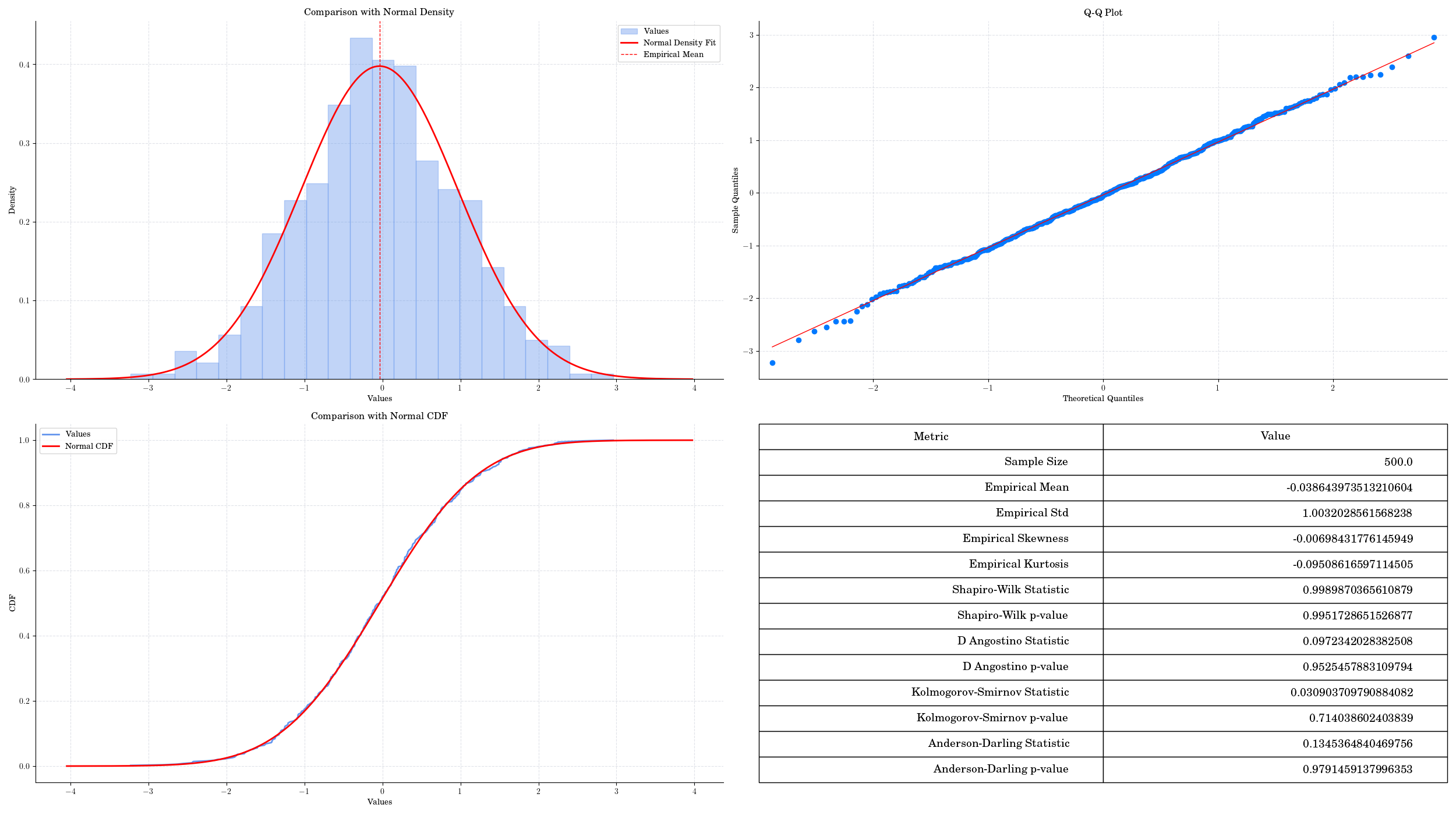
# Testing our function with a sample from a normal distribution

np.random.seed(123)
normal_data = np.random.normal(0, 1, 500)
normality_test(normal_data, visualise = True, colour ='cornflowerblue')

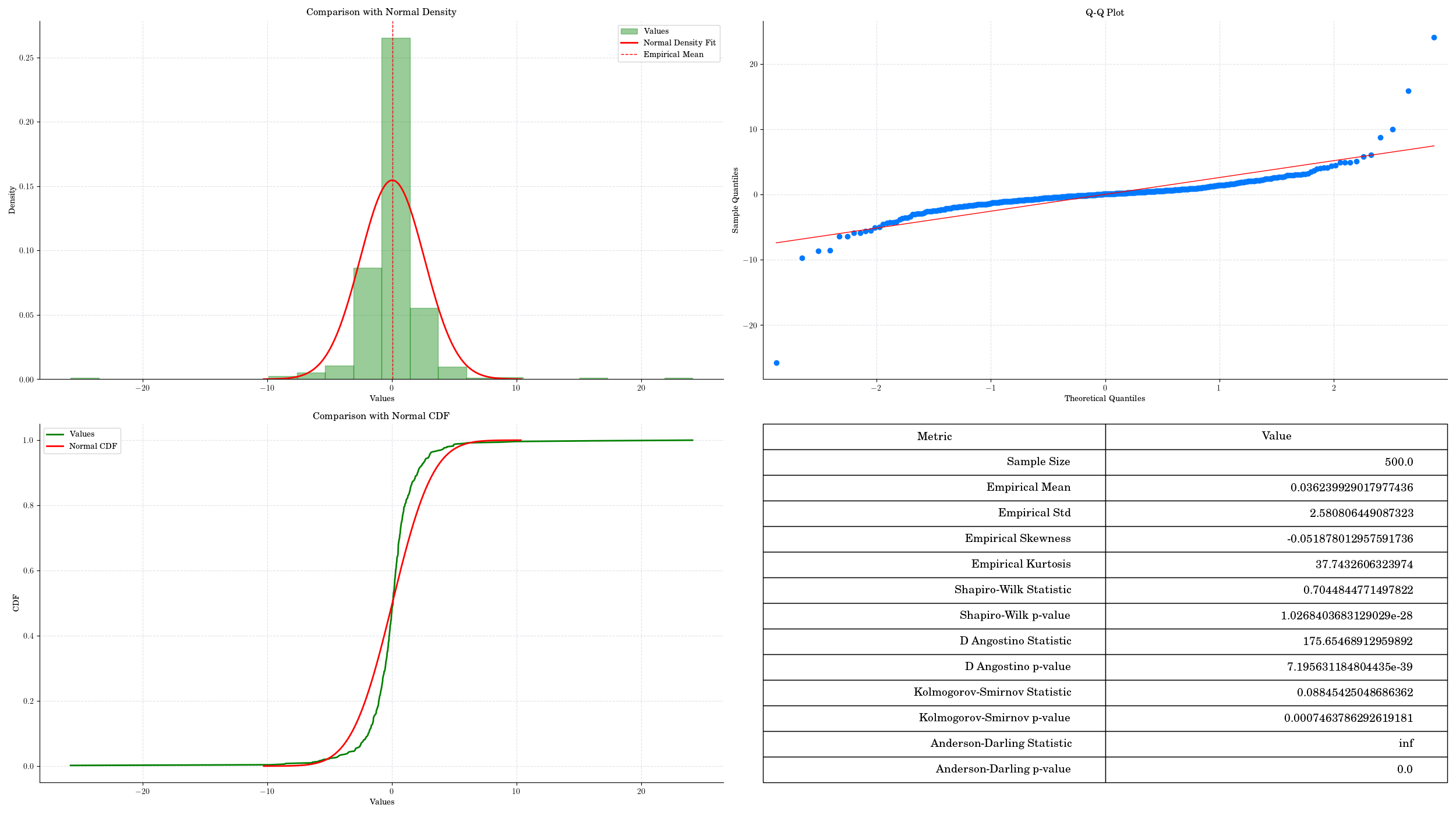
t_data = np.random.standard_t(2, 500)
normality_test(t_data, visualise = True, colour ='green')

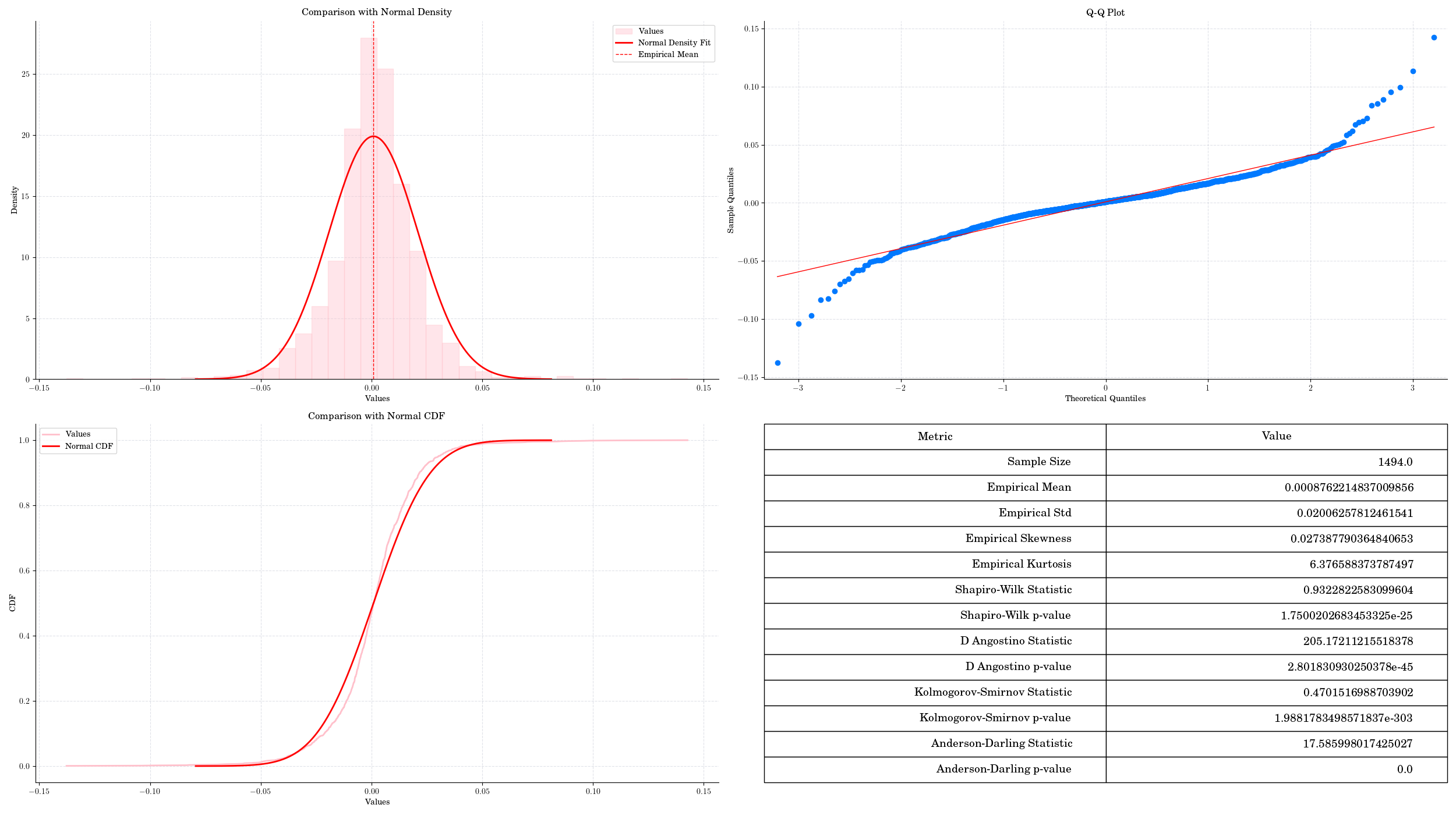
ticker = "AAPL"
data = yf.download(ticker, start="2020-01-01", progress=False, auto_adjust=False)
prices = data["Close"]
log_returns = np.log(prices / prices.shift(1)).dropna()
normality_test(log_returns[ticker], visualise=True, colour ='pink')